Non-Collusive and Collusive Oligopoly (With Diagram)

Let us learn about Non-Collusive and Collusive Oligopoly.

Non-Collusive Oligopoly: Sweezy’s Kinked Demand Curve Model:

One of the important features of oligopoly market is price rigidity. And to explain the price rigidity in this market, conventional demand curve is not used. The idea of using a non-conventional demand curve to represent non-collusive oligopoly (i.e., where sellers compete with their rivals) was best explained by Paul Sweezy in 1939. Sweezy uses kinked demand curve to describe price rigidity in oligopoly market structure.

The kink in the demand curve stems from the asymmetric behavioural pattern of sellers. If a seller increases the price of his product, the rival sellers will not follow him so that the first seller loses a considerable amount of sales. In other words, every price increase will go unnoticed by rivals.

On the other hand, if one firm reduces the price of its product other firms will follow the first firm so that they must not lose customers. In other words, every price will be matched by an equivalent price cut. As a result, the benefit of price cut by the first firm will be inconsiderable. As a result of this behavioural pattern, the demand curve will be kinked at the ruling market price.

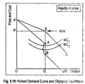
Suppose, the prevailing price of an oligopoly product in the market is QE or OP of Fig. 5.19. If one seller increases the price above OP, rival sellers will keep the prices of their products at OP. As a result of high price charged by the firm, buyers will shift to products of other sellers who have kept their prices at the old level. Consequently, sales of the first seller will drop considerably.

That is why demand curve in this zone (dE) is relatively elastic. On the other hand, if a seller reduces the price of his product below QE, others will follow him so that demand for their products does not decline. Thus, demand curve in this region (i.e., ED) is relatively inelastic. This behavioural pattern thus explains why prices are inflexible in the oligopoly market — even if demand and costs change.

The kink in the demand curve at point E results in a discontinuous MR curve.

The MR curve has two segments :

At output less than OQ the MR curve (i.e., dA) will correspond to DE portion of AR curve, and, for output larger than OQ, the MR curve (i.e., BMR) will correspond to the demand curve ED. Thus, discontinuity in MR curve occurs between points A and B. In other words, between these two points, MR curve is vertical.

Equilibrium is achieved when MC curve passes through the discontinuous portion of the MR curve. Thus the equilibrium output is OQ, to be sold at a price OP.

Suppose, costs rise. As a result, MC curve will shift up from MC₁ to MC₂. The resulting price and output remain unchanged at OP and OQ, respectively. This fact explains stickiness of prices. In other words, in oligopolistic industries price is more stable than costs.

At first sight, the model seems to be attractive since it explains the behaviour of firms realistically. But the model has certain limitations. Firstly, it does not explain how the ruling price is determined. It explains that the demand curve has a kink at the ruling price.

In this sense, it is not a theory of pricing. Secondly, price rigidity conclusion is not always tenable. Empirical evidence suggests that higher costs force a further price rise above the kink. Despite these limitations, the model is popular among textbook authors.

Collusive Oligopoly Model: Price Leadership Model:

Non-collusive oligopoly model (Sweezy’s model) presented in the earlier section is based on the assumption that oligopoly firms act independently even though firms are interdependent in the market. A vigorous price competition may result in uncertainty.

The question that arises now is: how do oligopoly firms remove uncertainty? In fact, firms enter into pricing agreements with each other instead of adopting competition or price war with each other. Such agreement—both explicitly (or formal) and implicit (or informal)—may be called collusion.

Always, every firm has the inclination to achieve more strength and power over the rival firms. As a result, in the oligopolist industry, one finds the emergence of a few powerful competitors who cannot be eliminated easily by other powerful firms.

Under the circumstance, some of these firms act together or collude with each other to reap maximum advantage. In fact, in oligopolist industry, there is a natural tendency for collusion. The most important forms of collusion are: price leadership cartel and merger and acquisition.

When a formal collusive agreement becomes difficult to launch, oligopolists sometimes operate on informal tacit collusive agreements. One of the most common form of informal collusion is price leadership. Price leadership arises when one firm—may be a large as well as dominant firm—initiates price changes while other firms follow.

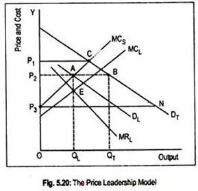
An example of dominant firm price leadership is shown in Fig. 5.20 where D_T is the industry demand curve. Since small firms follow the leader—the dominant firm—they behave as “price-takers”. MCs is the horizontal summation of the MC curves of all small firms.

Suppose, the dominant firm sets the price at OP₁ (where D_T and MCs intersect each other at point C). The small firms meet the entire demand P₁C at the price OP₁. Thus, the dominant firm has nothing to sell in the market. At a price of OP₃, the small firm will supply nothing. It is obvious that price will be set in between OP₁ and OP₃ by the leader.

The demand curve faced by the leader firm of the oligopoly industry is determined for any price—it is the horizontal distance between industry demand curve, D_T, and the marginal cost curves of all small firms, MC_S. In Fig. 5.20, D_L is the leader’s demand curve and the corresponding MR curve is MR_L.

Being a leader in the industry, the dominant firm’s supply curve is represented by the MC_L curve. Since it enjoys a cost advantage, its MC curve lies below the MC_S curve.

A dominant firm maximizes profit at point E where its MC_L and MR_L intersect each other. The corresponding output of the price leader is OQ_L. Price thus determined is OP₂. Small firms accept this price OP₂ and sell Q_LQ_T (=AB) amount – industry demand the OQ_T output.

In actual practice, the analysis of price leadership is complicated, particularly when new firms enter the industry and try to become the leader or dominant.

Collusive Oligopoly—Merger and Acquisition:

Another method to remove price war among oligopoly firms is merger. Merger may be defined as the consolidation of two or more independent firms under single ownership. When a firm purchases assets of another firm, acquisition takes place. Merger and acquisition take place because the management comes to a conclusion that a consolidated firm is powerful than the sum of individual firms.

Since basically the difference between cartel and merger is a legal one, we won’t consider mergers and acquisitions. The marginalistic principle applied in the case of profit maximizing cartel is also applicable in the case of merger.

Conclusion:

Can we make some definite conclusions from the oligopolistic market structure? Though one can make unambiguous predictions about perfect competition as well as monopoly, no such predictive element of an oligopolistic competition exists. It is, thus, a perplexing market structure. One important characteristic of an oligopoly market is interdependence among sellers.

Each seller’s price-output decision is influenced by the perceptions of countermoves of rival sellers.

Given the large number of possible reactions, we come up with different models based on different assumptions about the behaviour of the rival sellers, the extent and form of exit and entry, the likelihood of collusion between firms. ‘Unfortunately, economic theory does not suggest which assumptions to use. In any event, each of these theories must ultimately stand or fall on its predictive powers’.