Price Determination under Oligopoly: Non-Collusive and Collusive

In this article we will discuss about Non-Collusive and Collusive Price Determination under Oligopoly. 

The Sweezy Model of Kinked Demand Curve (Rigid Prices) (Non-Collusive Oligopoly):

In his article published in 1939, Prof. Sweezy presented the kinked demand curve analysis to explain price rigidities often observed in oligopolistic markets. Sweezy assumes that if the oligopolistic firm lowers its price, its rivals will react by matching that price cut in order to avoid losing their customers.

Thus the firm lowering the price will not be able to increase its demand much. This portion of its demand curve is relatively inelastic.

On the other hand, if the oligopolistic firm increases its price, its rivals will not follow it and change their prices. Thus the quantity demanded of this firm will fall considerably. This portion of the demand curve is relatively elastic. In these two situations, the demand curve of the oligopolistic firm has a kink at the prevailing market price which explains price rigidity.

Its Assumptions:

The kinked demand curve hypothesis of price rigidity is based on the following assumptions:

(1) There are few firms in the oligopolistic industry.

(2) The product produced by one firm is a close substitute for the other firms.

(3) The product is of the same quality. There is no product differentiation.

(4) There are no advertising expenditures.

(5) There is an established or prevailing market price for the product at which all the sellers are satisfied.

(6) Each seller’s attitude depends on the attitude of his rivals.

(7) Any attempt on the part of a seller to push up his sales by reducing the price of his product will be counteracted by other sellers who will follow his move.

(8) If he raises the price, others will not follow him; rather they will stick to the prevailing price and cater to the customers, leaving the price-raising seller.

(9) The marginal cost curve passes through the dotted portion of the marginal revenue curve so that changes in marginal cost do not affect output and price.

The Model:

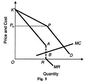
Given these assumptions, the price-output relationship in the oligopolist market is explained in Figure 5 where KPD is the kinked demand curve and OP_o the prevailing price in the oligopoly market for the OR product of one seller. Starting from point P, corresponding to the current price OP_o, any increase in price above it, will considerably reduce his sales, for his rivals are not expected to follow his price increase.

This is so because the KP portion of the kinked demand curve is elastic, and the corresponding portion KA of the MR curve is positive. Therefore, any price – increase will not only reduce his total sales but also his total revenue and profit.

On the other hand if the seller reduces the price of the product below OP_o (or P) his rivals will also reduce their prices. Though he will increase his sales, his profit would be less than before. The reason is that the PD portion of the kinked demand curve below P is less elastic and the corresponding part of marginal revenue curve below R is negative.

Thus in both the price-raising and price-reducing situations the seller will be a loser. He would stick to the prevailing market price OP_o which remains rigid. In order to study the working of the kinked demand curve, let us analyse the effect of changes in cost and demand conditions on price stability in the oligopolistic market.

Changes in Costs:

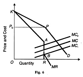
In oligopoly under the kinked demand curve analysis, changes in costs within a certain range do not affect the prevailing price. Suppose the cost of production falls so that the new MC curve is MC₁ to the right, as in Figure 6.

It cuts the MR curve in the gap AB so that the profit- maximising output is OR which can be sold at OP_o price. It should be noted that with any cost reduction the new MC curve will always cut the MR curve in the gap because as costs fall the gap AB continues to widen due to two reasons:

 

(1) As costs fall, the upper portion KP of the demand curve becomes more elastic because of the greater certainty that a price rise by one seller will not be followed by rivals and his sales would be considerably reduced.

(2) With the reduction in costs the lower portion PD of the kinked curve becomes more inelastic, because of the greater certainty that a price reduction by one seller will be followed by the other rivals.

Thus the angle KPD tends to be a right angle at P and the gap AB widens so that any AC curve below point A will cut the marginal revenue curve inside the gap. The net result is the same output OR at the same price OP_o and large profits for the oligopolistic sellers.

In case the cost of production rises the marginal cost curve will shift to the left of the old curve MC as MC_2. So long as the higher MC curve intersects the MR curve within the gap up to point A, the price situation will be rigid.

However, with the rise in costs the price is not likely to remain stable indefinitely and if the Ml curve rises above point A, it will intersect the MC curve in the portion KA so that a lesser quantity is sold at a higher price.

We may conclude that there may be price stability under oligopoly even when costs change so long as the MC curve cuts the MR curve in its discontinuous portion. However, chances of the existence of price-rigidity are greater where there is a reduction in costs than there is a rise in costs.

Changes in Demand:

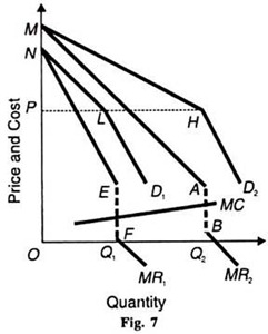
We now explain price rigidity where there is a change in demand with the help of Figure 7, D₂ is the original demand curve, MR₂ is its corresponding marginal revenue curve and MC is the marginal cost curve. Suppose there is a decrease in demand shown by D₁ curve and MR₁ is its marginal revenue curve.

When demand decreases, a price-reduction move by one seller will be followed by other rivals. This will make LD₁ the lower portion of the new demand curve, more inelastic than the lower portion HD₂ of the old demand curve.

This will tend to make the angle at L approach a right angle. As a result, the gap EF in MR₁ curve is likely to be wider than the gap AB of the MR₂ curve. The marginal cost curve MC will, therefore, intersect the lower marginal revenue curve MR₁ inside the gap EF, thus indicating a stable price for the oligopolistic industry.

Since the level of the kinks H and L of the two demand curves remains the same, the same price OP is maintained after the decrease in demand. But the output level falls from OQ₂ to OQ₁. This case can be reversed to show increase in demand by taking D₁ and MR₁ as the original demand and marginal revenue curves and D₂ and MR₂ as the higher demand and marginal revenue curves respectively.

The price OP is maintained but the output rises from OQ₁ to OQ. So long as the MC curve continues to intersect the MR curve in the discontinuous portion, there will be price rigidity.

However, if demand increases, it may lead to a higher price. When demand increases, a seller would like to raise the price of the product and others are expected to follow him. This will tend to make the upper portion MH of the new demand curve elastic than the NL portion of the old curve.

Thus the angle at H becomes obtuse, away from the right angle. The gap AB in the MR₂ curve becomes smaller and the MC curve intersects the MR₂ curve above the gap, indicating a higher price and lower output. If, however, the marginal cost curve passes through the gap of MR₂, there is price stability.

Conclusion:

The whole analysis of the kinked demand curve points out that price rigidity in oligopolistic markets is likely to prevail if there is a price reduction move on the part of all sellers. Changes in costs and demand also lead to price stability under normal conditions so long as the MC curve intersects the MR curve in its discontinuous portion.

But price increase rather than price rigidity may be found in response to rising cost or increased demand.

Reasons for Price Stability:

There are a number of reasons for price rigidity in certain oligopoly markets.

(1) Individual sellers in an oligopolistic industry might have learnt through experience the futility of price wars and thus prefer price stability.

(2) They may be content with the current prices, outputs and profits and avoid any involvement in unnecessary insecurity and uncertainty.

(3) They may also prefer to stick to the present price level to prevent new firms from entering the industry.

(4) The sellers may intensify their sales promotion efforts at the current price instead of reducing it. They may view non-price competition better than price rivalry.

(5) After spending a lot of money on advertising his product, a seller may not like to raise its price to deprive himself of the fruits of his hard labour. Naturally, he would stick to the going price of the product.

(6) If a stable price has been set through agreement or collusion, no seller would like to disturb it, for fear of unleashing a price war and thus engulfing himself into an era of uncertainty and insecurity.

(7) It is the kinked demand curve analysis which is responsible for price rigidity in oligopolistic markets.

Its Shortcomings:

But the theory of kinked demand curve in oligopoly pricing is not without shortcomings.

(1) Even if we accept all its assumptions it is not likely that the gap in the marginal revenue curve will be wide enough for the marginal cost curve to pass through it. It may be shortened even under conditions of fall in demand or costs, thereby making price unstable.

(2) One of its major shortcomings, according to Professor Stigler, is that “the theory does not explain why prices that have once changed should settle down, again acquire stability, and gradually produce a new kink.” For instance in Figure 6 the kink occurs at P because OP_o is the prevailing price. But the theory does not explain the forces that established the initial price OP_o.

(3) Price stability may be illusory because it is not based on the actual market behaviour. Sales do not always occur at list prices. There are often deviations from posted prices because of trade-ins, allowances and secret price concessions. The oligopolistic seller may outwardly keep the price stable but he may reduce the quality or quantity of the product. Thus price stability becomes illusory.

(4) Moreover, it is not possible to statistically compile actual sales prices in the case of many products that may reflect stable prices for them. It is, therefore, doubtful that price stability actually exists in oligopoly.

(5) Critics point out that the kinked demand curve analysis holds during the short-run, when the knowledge about the reactions of rivals is low. But it is difficult to guess correctly the rivals’ reactions in the long-run. Thus the theory is not applicable in the long-run.

(6) According to some economists, the kinked demand curve analysis applies to an oligopolistic industry in its initial stages or to that industry in which new and previously unknown rivals enter the market.

(7) The kinked demand curve analysis is based on two assumptions: first, other firms will follow a price cut and, second, they will not follow a price rise. Stigler has shown on empirical evidence that in an inflationary period the rise in output prices is not confined only to one firm but is industry-wide. So all firms having similar costs will follow one another in raising price.

(8) Economists have concluded from this that the kinked demand curve analysis is applicable only under depression. For in an inflationary period when demand increases, the oligopolistic firm will raise price and other firms will also follow it.

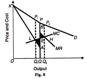
In such a situation, the demand curve of the oligopolist will have an inverted kink. This reverse kink is based on his expectation that all his competitors will follow him when he raises the price of his product, but none will follow a price cut because of inflationary condition.

This is illustrated in Figure where KPD is the reverse kinked de­mand curve. Its corresponding marginal revenue curve is KABM which is composed of KA and BM, and the AB portion is its gap. The curve MC passes through all the three portions of this curve at L, E and H respectively.

The areas ALE and ВНЕ are of uncertainty. Whether the firm decides to continue production at L, E and H depends on the balance of gain and loss. A movement from L to E results in a loss because MC>MR. A movement from E to H results in a gain because MR>MC. If the firm raises the price to Q₁P₁ and lowers the output to OQ₁ and moves from E to L, it would reduce the loss. If it lowers the price to Q₂P₂, and raises the output to OQ₂ and moves from E to H, it would increase the gain. The firm would move to the larger area of gain. Thus there would be no price rigidity.

(9) Stigler’s empirical evidence further shows that cases in oligopoly industries where the number of sellers is either very small or somewhat large, the kinked demand curve is not likely to be there. Thus the empirical evidence does not support the existence of a kink.

“However”, as pointed out by Professor Baumol, “the analysis does show how the oligopolistic firm’s view of competitive reaction patterns can affect the changeability of whatever price it happens to be charging.”

2. Collusive Oligopoly:

Collusive oligopoly is a situation in which firms in a particular industry decide to join together as a single unit for the purpose of maximising their joint profits and to negotiate among themselves so as to share t e market.

The former is known as the joint profit maximisation cartel and the latter as the market-sharing cartel. There is another type of collusion, known as leadership, which is based on tacit agreements. Under it, one firm acts as the price leader and fixes the price for the product while other firms follow it. Price leadership is of three types: low-cost firm, dominant firm, and barometric.

(A) Cartels:

A cartel is an association of independent firms within the same industry. The cartel follows common policies relating to prices, outputs, sales and profit maximisation and distribution of products Cartels may be voluntary or compulsory and open or secret depending upon the policy of the government with regard to their formation.

Thus cartels have many forms and use many devices in order to follow varied common policies depending upon the type of the cartel.

We discuss below the two most common types of cartels:

(1) Joint profit maximisation or perfect cartel; and

(2) Market-sharing cartel.

1. Joint Profit Maximisation Cartel:

The uncertainty to be found in an oligopolistic market provides an incentive to rival firms to form a perfect cartel Perfect cartel is an extreme form of perfect collusion. In this, firms producing a homogeneous product form a centralised cartel board in the industry.

The individual firms surrender their price-output decisions to this central board. The board determines output quotas for its members, the price to be charged and the distribution of industry profits. Since the central board manipulates prices, outputs, sales and distribution of profits, it acts like a single monopoly whose main aim is to maximise the joint profits of the oligopolistic industry.

Its Assumptions:

The analysis of joint profit maximisation cartel is based on the following assumptions:

1. Only two firms A and В are assumed in the oligopolistic industry that forms the cartel.

2. Each firm produces and sells a homogeneous product that is a perfect substitute for each other.

3. The number of buyers is large.

4. The market demand curve for the product is given and is known to the cartel.

5. The cost curves of the firms are different but are known to the cartel.

6. The price of the product determines the policy of the cartel.

7. The cartel aims at joint profit maximisation.

Joint Profit Maximisation Solution:

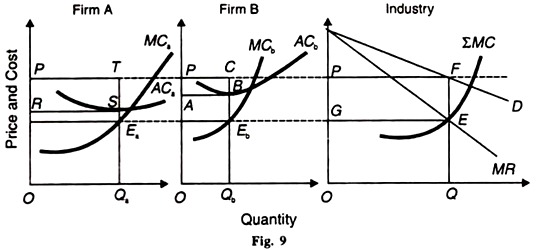
Given these assumptions, and given the market demand curve and its corresponding MR curve, joint profits will be maximised when the industry MR equals the industry MC. Figure 9 illustrates this situation where D is the market (or cartel) demand curve and MR is its corresponding marginal revenue curve.

The aggregate marginal cost curve of the industry SMC is drawn by the lateral summation of the MC curves of firms A and B, so that SMC = MC_a+ MC_b.

The cartel solution that maximises joint profit is determined at point E where the SMC curve intersects the industry MR curve. Consequently, the total output is OQ which will be sold at price Qp = (Qf). As under monopoly, the cartel board will allocate the industry output by equating the industry MR to the marginal cost of each firm.

The share of each firm in the industry output is obtained by drawing a straight line from E to the vertical axis which passes through the curves MC_b and MC_a of firms В and A at points E_b and E_a respectively. Thus the share of firm A is OQ_a and that of firm В is OQ_b which equal the total output OQ (=OQ_a + OQ_b).

The price OP and the output OQ distributed between A and В firms in the ratio of OQ_a: OQ_b is the monopoly solution. Firm A with the lower costs sells a larger output OQ_a than the firm В with higher costs so that OQ_a > OQ _b. But this does not mean that A will be getting more profit than B. The joint maximum profit is the sum of RSTP and ABCP earned by A and В respectively.

It will be pooled into a fund and distributed by the cartel board according to the agreement arrived at by the two firms at the time of the formation of the cartel. A pooling agreement of this type will make it possible for both firms to maximise their joint profit provided the total profits earned by them independently do not exceed the former.

Advantages:

Perfect collusion by oligopolistic firms in the form of a cartel has certain advantages:

1. It avoids price wars among rivals.

2. The firms forming a cartel gain at the expense of customers who are charged a high price for the product.

3. The cartel operates like a monopoly organisation which maximises the joint profit of firms.

4. Joint profits are generally more than the total profits earned by them if they were to act independently.

Difficulties of a Cartel:

The above analysis is based on perfect collusion in which all firms relinquish their individual price- output decisions to a central board of the cartel which acts like a multi-plant monopolist. But this is only a theoretical possibility in the short-run because in practice the joint profit maximisation objective cannot be achieved by a cartel.

In the long-run, there are a number of difficulties faced by a cartel which tend to break it down.

They are as under:

1. It is difficult to make an accurate estimate of the market demand curve. Each firm thinks that its own demand curve is more elastic than the market demand curve because its product is a perfect substitute for the product of its rivals. Thus if the market demand curve is underestimated so will be its corresponding MR curve which will make the estimation of the market price inaccurate by the cartel.

2. Similarly, the estimation of the market MC curve may be inaccurate because of the supply of wrong data about their marginal costs by individual firms to the cartel. There is every possibility that the individual firms may supply low-cost data to the central cartel board in order to have a larger share of output and profits. This may ultimately lead to the breakdown of the cartel.

3. The formation of a cartel is a slow process which takes a long time for the agreement to arrive at by firms especially if their number is very large. In the meantime, there may be changes in the cost structure and market demand for the product. This renders the cartel agreement useless and it breaks down soon.

4. If a firm’s product is preferred more by consumers than that of the other members of the cartel, the market demand for it may be higher than the quota fixed by the cartel. It may, therefore, secretly sell more than its quota and if followed by other firms, the cartel will break down.

5. The larger the numbers of firms in a cartel, the less are its chances of survival for long because of the distrust, threatening and bargaining resorted to by them. The cartel will, therefore, break down.

6. In theory, the cartel-members agree on joint profit maximisation. But in practice, they seldom agree on profit distribution. Large firms want a lower price, a higher output quota and larger profits. So when such problems arise: in joint profit distribution in contravention of the cartel agreement, they lead to the breakdown of the cartel.

7. The price of the product fixed by the cartel cannot be changed even if the market conditions require it to be changed. This is because it takes a long time for the members to arrive at an agreed price. This stickiness of the price often leads to the breakdown of the cartel when some members defect from it.

8. Price stickiness gives rise to ‘chislers’ who secretly cut the price or violate the quota agreement. Such secret dealings by firms to raise their own profits tend to break down the cartel.

9. Unless all member firms in the cartel are strongly committed to cooperation, outside disturbances, such as a sharp fall in demand, may lead to the breakdown of the cartel.

10. When a cartel raises the price of the product and increases the profits of its members, it creates an incentive for new firms to enter the industry. Even if the entry of new firms is blockaded, it is only a short-run phenomenon because the success of the cartel will lead to the entry of firms in the long-run.

This will force the cartel to break down. If the new firms are allowed to enter the cartel, it will become unmanageable, increase the defectors and bring its end.

11. Some high-cost uneconomic firms may refuse to shut down or leave the cartel despite the cartel board’s request. This is likely to distort the profit maximisation level of the cartel and thus break it.

12. The cartel’s policy of fixing high price and restricting the quantity of the product may lead to the emergence of substitutes in the long-run. The other firms may invent and produce cheaper substitutes which may be accepted by consumers. This will tend to reduce the demand for the cartel’s product, make it more elastic, reduce its joint profits and thus break the cartel.

13. The cartel may not be able to maximise joint profits by not charging a very high price for fear of government interference and regulation.

14. Similarly, the cartel may not charge a very high price and maximise its joint profits in order to have a good public image or reputation.

15. Besides, it is more difficult to form and run a cartel for long in the case of a differentiated product than in the case of a homogeneous product. For, it is not possible to rationalise and sort out the differences in the qualities of the product.

Thus the chances are greater for individual firms to leave the cartel on account of personal bickering and antagonism of member firms over allotment of quotas and division of profits which are likely to affect adversely joint profit maximisation and end the cartel agreement.

2. Market-Sharing Cartel:

Another type of perfect collusion in an oligopolistic market is found in practice which relates to market-sharing by the member firms of a cartel. The firms enter into a market-sharing agreement to form a cartel “but keep a considerable degree of freedom concerning the style of their output, their selling activities and other decisions.”

There are two main methods of market-sharing:

(a) Non-price competition; and

(b) Quota system.

They are discussed as under:

(a) Non-Price Competition Cartel:

The non-price competition agreement among oligopolistic firms is a loose form of cartel. Under this type of cartel, the low-cost firms press for a low price and the high-cost firms for a high price. But ultimately, they agree upon a common price below which they will not sell.

Such a price must allow them some profits. The firms can compete with one another on a non-price basis by varying the colour, design, shape, packing, etc. of their product and having their own different advertising and other selling activities. Thus each firm shares the market on a non-price basis while selling the product at the agreed common price.

This type of cartel is inherently unstable because if one low-cost firm cheats the other firms by charging a lower price than the common price, it will attract the customers of other member firms and earn larger profits. When other firms come to know of this, they will leave the cartel. A price war will start and ultimately the lowest-cost firm will remain in the industry.

In case the cost curves of the firms forming a cartel differ, the low-cost firms may not stick to the common price. They may try to increase their share of the market by means of secret price concessions. They may also resort to better sales promotion methods.

Such policies tend to change their demand-cost conditions further. Consequently, price variations among firms become more common. Ultimately, the cartel agreement becomes a farce and a price war starts. This leads to the breaking up of the cartel agreement.

(b) Market Sharing by Quota Agreement:

The second method of market sharing is the quota agreement among firms. All firms in an oligopolistic industry enter into collusion for charging an agreed uniform price. But the main agreement relates to the sharing of the market equally among member firms so that each firm gets profits on its sales.

Its Assumptions:

This analysis is based on the following assumptions:

1. There are only two firms that enter into market-sharing agreement on the basis of the quota system.

2. Each firm produces and sells a homogeneous product which is a perfect substitute for each other.

3. The number of buyers is large.

4. The market demand curve for the product is given and known to the cartel.

5. Each firm has its own demand curve having the same elasticity as that of the market demand curve.

6. The cost curves of the two firms are identical.

7. Both firms share the market equally.

8. Each sells the product at the agreed uniform price.

9. There is no threat of entry by new firms.

Market-Sharing Solution:

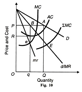
Given these assumptions, the equal market sharing between the two firms is explained in terms of Figure 10 where D is the market demand curve and d/MR is its corresponding MR curve. S MC is the aggregate MC curve of the industry. The SMC curve intersects the d/MR curve at point E which determines QA (=OP) price and total output OQ for the industry. This is the monopoly solution in the market-sharing cartel.

How will the industry output be shared equally between the two firms? Now assume that the d/MR is the demand curve of each firm and mr is its corresponding MR curve.

AC and MC are their identical cost curves. The MC curve intersects the mr curve at point e so that the profit maximisation output of each firm is Oq. Since the total output of the industry is OQ which is equal to 2 x Oq= (OQ=2Oq), it is equally shared by the two firms as per the quota agreement between them.

Thus each sells Oq output at the same price qB (= OP) and earns RP per unit profit. The total profit earned by each firm is RP x Oq and by both is RP ×-2Oq or RP x OQ. However, in actuality, there are more than two firms in an oligopolistic industry which do not share the market equally.

Moreover, their cost curves are also not identical. In case their cost curves differ, their market shares will also differ. Each firm will charge an independent price in accordance with its own MC and MR curves. They may not sell the same quantity at the agreed common price.

They may be charging a price slightly above or below the profit maximisation price depending upon its cost conditions. But each will try to be nearest the profit maximisation price. This will ultimately lead to the breaking up of the market sharing agreement.

With Threat of Entry:

So far our analysis has been confined to collusive oligopoly without any threat of entry of new firms in the industry. Suppose there is a constant threat of entry into the oligopolistic industry. In that case if the firms agree on the price OP, new firms will enter the industry, reduce their sales and profits.

This may ultimately lead to excess capacity and uneconomic firms in the industry. The existence of excess capacity and uneconomic firms will raise the average costs AC to the level of В (not shown in Figure (10) and the firms will be earning only normal profits. Each firm will sell less than Oq.

If the existing oligopolists are wiser, they may forestall entry by charging a price lower than the profit maximisation price OP In this way, the collusive oligopolists by charging a lower price in the present will be earning larger profits in the long-run, and continue their exclusive control over the market by keeping the new entrants out for ever.

We may conclude that perfect collusive oligopoly pricing has not any set pattern of price behaviour. The resultant price and output will depend upon the reaction of the collusive oligopolists towards the profit maximisation price and their attitude towards the existing and potential rivals.

(B) Price Leadership:

Price leadership is imperfect collusion among the oligopolistic firms in an industry when all firms follow the lead of one big firm. There is a tacit agreement among the firms to sell the product at a price set by the leader of the industry (i.e. the big firm).

Sometimes there is a formal meeting and a definite agreement with the leader-firm. If the products are homogeneous, a uniform price is established. In the case of differentiated products, prices can be also uniform.

Whatever price changes take place, the leader announces from time to time, and the other firms follow him. In America, examples of price leadership industries are: biscuits, cement, cigarettes, flour, fertilizers, petroleum, milk, rayon, steel, etc. They relate both to pure and differentiated oligopoly.

Price leadership is of various types. But there are three most common price leadership models which we discuss below.

1. The Low-Cost Price Leadership Model:

In the low-cost price leadership model, an oligopolistic firm having lower costs than the other firms sets a lower price which the other firms have to follow. Thus the low-cost firm becomes the price leader.

There are two low-cost price leadership models:

(1) With equal market shares, and

(2) With unequal market shares.

We explain them as under:

Assumptions:

The low-cost firm model is based on the following assumptions:

1. There are two firms A and B.

2. Their costs differ. A is the low-cost firm and В is the high-cost firm.

3. They have identical demand and MR curves. The demand curve faced by them is 1/2 of the market demand curve.

4. The number of buyers is large.

5. The market industry demand curve for the product is known to both the firms.

The Model:

(1) Equal Market Shares:

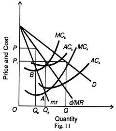
Given these assumptions, both firms enter into a tacit agreement whereby the high-cost firm В will follow the price set by the price leader firm A and to share the market equally. The price policy to be followed by both is illustrated in Figure 11.

D is the industry demand curve and d/MR is its corresponding marginal revenue curve which is the demand curve for both the firms and mr is their marginal revenue curve. The cost curves of the low- cost firm A are AC_a and MC_a and of the high- cost firm В is AC_b and MC_b.

If the two firms were to act independently, the high cost firm В would charge OP price per unit and sell OQ_b quantity, as determined by point В where its MC_b curve cuts the mr curve. Similarly, the low-cost firm A would charge OP₁ price per unit and sell OQ_a quantity, as determined by point A where its MC_a curve cuts the mr curve.

As there is a tacit agreement between о the two firms, the high-cost firm В has no choice but to follow the price leader firm A.

It will, therefore, also sell OQ_a quantity at a lower price OP₁ even though it will not be earning maximum profits.

On the other hand, the price leader A will earn much higher profits at OP₁ price by selling OQ_a quantity.

Since both A and В sell the same quantity OQ_a the total market demand OQ is equally divided between the two, OQ = 2 OQ_a. But if firm В sticks to OP price, its sales will be zero because the product being homogeneous, all its customers will shift to firm A.

The price-leader firm A can, however, drive firm В out of the market by setting a lower price than OP₁ lower than the average cost AC_b of firm B. Firm A would become a monopoly firm. But in such a situation it will have to face legal problems. Therefore, it will be in its interest to fix OP, price and tolerate firm В in order to share the market equally and maximise its profits.

(2) Unequal Market Shares:

In the case of the price leadership model with unequal market shares, the two firms will have different demand curves along with their different cost curves. The low-cost firm’s demand curve will be more elastic than that of the high-cost firm. The high-cost firm would maximise its profits by selling less at a higher price while the low-cost firm would sell more at a lower price and maximise its profits.

If they enter into a common price agreement, it would be in the interest of the high-cost firm to sell more quantity at a lower price set by the price leader by earning a little less than the maximum profits. But this is only possible so long as the price set by the leader covers the AC of the high- cost firm.

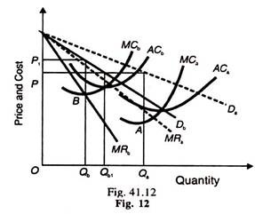
The price leadership model with unequal market shares is illustrated in Figure 12, where the market demand curve is not shown to simplify the analysis. In the figure, D_a is the demand curve of the low-cost firm A and MR_a is its marginal revenue curve.

The demand curve and MR curve of the high- cost firm В are D_b and MR_b. The low-cost firm A sets the price OP and the quantity OQ_a when its MC_a curve cuts its MR curve at point A.

The price OP₁ and the quantity OQ_b of the high-cost firm В are determined when its MC_b curve cuts its MR_b curve at point B. Following the price leader firm A, when firm В accepts the price OP, it sells more quantity OQ_b1 and earns less than maximum profits.

It will pay the follower firm to sell this quantity at OP price so long as this price covers its average cost. If it does not follow the leader firm and tries to sell OQ_b quantity at its profit maximisation price OP₁ it will have to close down because its customers will switch over to the leader firm which charges low price OP.

However, if there is no agreement for sharing the market between the leader and the follower firms, the follower can adopt the price of the leader (OP) but produce a lower quantity (less than OQ_b1) than required to maintain the price in the market, and thus push the leader to a non-profit maximisation position by producing less output.

2. The Dominant Firm Price Leadership Model:

This is a typical case of price leadership where there is one large dominant firm and a number of small firms in the industry. The dominant firm fixes the price for the entire industry and the small firms sell as much product as they like and the remaining market is filled by the dominant firm itself. It will, therefore, select that price which brings more profits to it.

Assumptions:

This model is based on the following assumptions:

(1) The oligopolistic industry consists of a large dominant firm and a number of small firms.

(1) The dominant firm sets the market price.

(3) All other firms act like pure competitors, which act as price takers. Their demand curves are perfectly elastic for they sell the product at the dominant firm’s price.

(4) The dominant firm alone is capable of estimating the market demand curve for the product.

(5) The dominant firm is in a position to predict the supplies of other firms at each price set by it.

The Model:

Given these assumptions, when each firm sells its product at the price set by the dominant firm, its demand curve is perfectly elastic at that price. Thus its marginal revenue curve coincides with the horizontal demand curve.

The firm will produce that output at which its marginal cost equals marginal revenue. The MC curves of all the small firms combined laterally establish their aggregate supply curve. All these firms behave competitively while the dominant firm behaves passively. It fixes the price and allows the small firms to sell all they wish at that price.

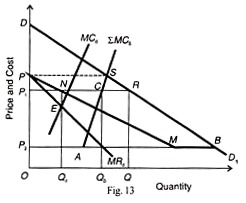
The case of price leadership by the dominant firm is explained in terms of Figure 13 where DD is the market demand curve. SMC_s are the aggregate supply curve of all the small firms. By subtracting SMC_s from DD₁ at each price, we get the demand curve faced by the dominant firm, PNMBD₁ which can be drawn as follows.

Suppose the dominant firm sets the price OP. At this price, it allows the small firms to meet the entire market demand by supplying PS quantity. But the dominant firm would supply nothing at the price OP. Point P is, therefore, the starting point of its demand curve.

Now take a price OP₁ less than OP. The small firms would supply P₁C (=OQ_s) output at this price OP₁ when their SMC_s curve cuts their horizontal demand curve P₁R at point C. Since the total quantity demanded at OP₁ price is P₁R (=OQ) and the small firms supply P₁C quantity, CR (=Q_SQ) quantity would be supplied by the dominant firm.

By taking P₁N = CR on the horizontal line P₁R, the dominant firm’s supply becomes P₁N (=OQ_d). Thus we derive point N on the dominant firm’s demand curve by subtracting the horizontal distance from point P₁ to N from the demand curve DD_1.

Since the small firms supply nothing at prices below OP₂ because their SMC_s curve exceeds this price, the dominant firm’s demand curve coincides with the horizontal line P₂B over the range MB and then with the market demand curve over the segment BD₁.

Thus the dominant firm’s demand curve is PNMBD₁. The dominant firm will maximise its profits at that output where its marginal cost curve MC, cuts its MR_d, the marginal revenue curve. It establishes the equilibrium point E at which the dominant firm sells OQ_d output at OP₁ price. 

The small firms will sell OQ_s output at this price for the marginal cost curve SMC_S, of the small firms equals the horizontal price line P ₁ R at C.

The total output of the industry will be OQ = OQ _d + OQ_s. If OP₂ price is set by the dominant firm, the small firms would sell P₂A and the dominant firm AB. In case a price below OP₂ is set the dominant firm would meet the entire industry demand and the sales of the small firms would be zero.

The above analysis shows that the price-quantity solution is stable because the small firms behave passively as price-takers. But this does not mean that the dominant firm charges the same price that is charged by a monopolist operating in the same market.

However, the real test of a dominant firm’s price leadership is the extent to which the other firms follow its lead. The moment the firms cease to follow the price leader, the model breaks down. Besides, if the other firms have different cost curves, the same price may not maximise short-run profits for all the firms.

The dominant-firm model of price leadership can have a number of variations. There may be two or more large firms among a number of small firms which may enter into collusion for sharing the market at various prices. There may be product differentiation. Nevertheless, the conclusions arrived at help to explain Price- output policies in all such situations.

3. The Barometric Price Leadership Model:

The barometric price leadership is that in which there is no leader firm as such but one firm among the oligopolistic firms with the wisest management which announces a price change first which is followed by other firms in the industry. The barometric price leader may not be the dominant firm with the lowest cost or even the largest firm in the industry.

It is a firm which acts like a barometer in forecasting changes in cost and demand conditions in the industry and economic conditions in the economy as a whole. On the basis of a formal or informal tacit agreement, the other firms in the industry accept such a firm as the leader and follow it in making price changes for the product.

The barometric price leadership develops due to the following reasons:

1. As a reaction to the earlier experience of violent price changes and cut-throat competition among oligopolistic firms, they accept one firm as the price leader.

2. Most firms do not possess the expertise to calculate cost and demand conditions of the industry, so they leave their estimation to one leader firm which has the ability to do so.

3. Oligopolistic firms accept one among them as the barometric leader firm which possesses better knowledge and predictive power about changes in direct costs or style and quality changes and changes in the economic conditions as a whole. It is not essential that a firm selected as the barometric leader must belong to the industry. Even a firm not belonging to the industry may be chosen as the barometric leader.