Slopes of Functions of Optimization (With Examples)

In economics it is important to know the rate at which a variable changes in response to a change in another variable, the slope of a variable measures this rate.

For example, it is important to know the rate at which quantity demanded of a commodity changes in response to a change in price of a commodity. In the field of economics we find both linear and non­linear functions.

1. Slope of a Linear Function:

Consider the following linear function:

y = ƒ(X) = 2 + 0.5 X

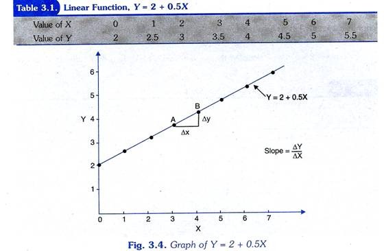
In Table 3.1 we have calculated the values of the variable V by taking different values of X such as 1, 2, 3, 4 etc. Further, we have plotted the different values of Table 3.1 on a graph shown in Fig. 3.4. The slope of the function. (Y = 2 + 0.5X) between two points, say, A and B

In Figure 3.4 is given by the ratio of change in Y to the change in X. That is, slope = ∆Y/∆X

For example, at point A of the given function value of variable X is 3 and corresponding to it the value of variable Y is 3.5. When value of X rises from 3 to 4, value of Y increases from 3.5 to 4. Thus, the slope of the function (Y = 2 + 0.5Y) is:

∆Y/∆X= 4- 3.5/ 4-3 = 0.5 /1 = 0.5

This implies that value of Y increases by 0.5 when value of X increases by 1. It should be noted that slope of a linear function is constant throughout.

However, the slope of a linear function can be directly known from the linear function itself and for that purpose there is no need to plot the data. Consider the following linear function

Y = a + bX

It will be seen from this linear function that when the value of X is zero, the value of Y will be equal to a. Thus a is Y intercept. Further, in this function b is the coefficient of X and measures change in Y due to change in X, that is ∆Y/∆X. Thus, b represents the slope of the linear function. In linear function Y = 2 + 0.5X, 2 is the Y-intercept, that is, value of Y when X is zero, 0.5 is the b coefficient which measures the slope ∆Y /∆ X of the linear function.

2. Slope of a Non-linear Function:

We now turn to explain how slope of a non-linear function, say, a quadratic function (Y = a + bX + cX²) can be measured. On plotting the non-linear function in a graph, we get a non-linear curve.

Let us take the following specific quadratic function:

Y = 5 + 3X + X²

In Table 3.2 we have calculated the various values of Y by taking different values of X (0, 1, 2, 3, etc)

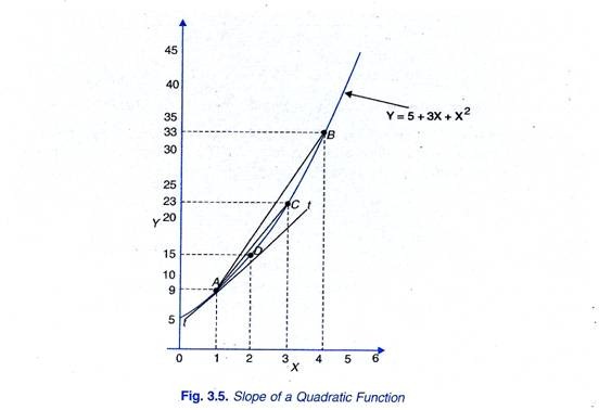
The data so obtained have been plotted to get a curve in Figure 3.5. It will be seen from this Figure 3.5 that slope of the line AB which connects two points A and Bona curve representing quadratic function can be measured by taking the change in the value of y divided by the change in value of X. At point A, value of X is 1 and the corresponding value of Y is 9 and at point B, the value of X is 4 to which the corresponding value is 33. Thus, here ∆X = 4 – 1 = 3 and ∆Y = 33 – 9 = 24.

Thus, the slope of the line AB is ∆Y/∆X= 24/3 =8

Similarly, slope of straight line AC in Fig 3.5 can be measured. Between two points A and C ∆X= 3-1 =2 ∆Y =23-9 = 14. Thus, the slop of straight line AC is

∆Y/∆X= 14/2=7

In a similar fashion, the slope of the straight line AD connecting points A and D on the non-linear quadratic function curve in Figure 3.5 is given by

∆Y/∆X= 15- 9 / 2-1 =6/1=6

It will thus be seen that as ∆X decreases; it was 3 between A and B, 2 between A and C and 1 between A and D, slope of the non-linear curve goes on declining. It was 8 of the line AB, 7 of the line AC and 6 of the line AD. As ∆X further decreases, slope of the line connecting two points of the non-linear curve will further decline,.

It should also be noticed that the slope of the straight line AD connecting points A and D is very close to the slope of the tangent drawn to the curve at point A. As ∆X becomes smaller and smaller slope of the line connecting the two points on a curve will become extremely close to the slope of the tangent drawn to the curve at point A. Therefore, the slope at a point on the non-linear function curve can he measured by the slope of a tangent drawn to the curve at that point.