Equilibrium of the Firm and the Industry in Long-Run

In the long run firms are in equilibrium when they have adjusted their plant so as to produce at the minimum point of their long-run AC curve, which is tangent (at this point) to the demand curve defined by the market price.

In the long run the firms will be earning just normal profits, which are included in the LAC.

If they are making excess profits new firms will be attracted in the industry; this will lead to a fall in price (a down- ward shift in the individual demand curves) and an upward shift of the cost curves due to the increase of the prices of factors as the industry expands.

These changes will continue until the LAC is tangent to the demand curve defined by the market price. If the firms make losses in the long run they will leave the industry, price will rise and costs may fall as the industry contracts, until the remaining firms in the industry cover their total costs inclusive of the normal rate of profit.

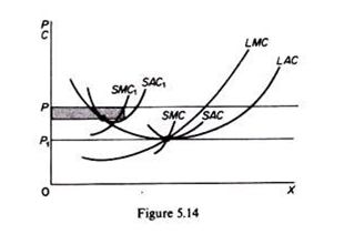
In figure 5.14 we show how firms adjust to their long-run equilibrium position. If the price is P, the firm is making excess profits working with the plant whose cost is denoted by SAC₁. It will therefore have an incentive to build new capacity and it will move along its LAC. At the same time new firms will be entering the industry attracted by the excess profits.

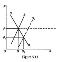
As the quantity supplied in the market increases (by the increased production of expanding old firms and by the newly established ones) the supply curve in the market will shift to the right and price will fall until it reaches the level of P₁ (in figure 5.13) at which the firms and the industry are in long-run equilibrium. The LAC in figure 5.14 is the final-cost curve including any increase in the prices of factors that may have taken place as the industry expanded.

The condition for the long-run equilibrium of the firm is that the marginal cost be equal to the price and to the long-run average cost

LMC = LAC = P

The firm adjusts its plant size so as to produce that level of output at which the LAC is the minimum possible, given the technology and the prices of factors of production. At equilibrium the short-run marginal cost is equal to the long-run marginal cost and the short-run average cost is equal to the long-run average cost. Thus, given the above equilibrium condition, we have

SMC = LMC = LAC = LMC = P = MR

This implies that at the minimum point of the LAC the corresponding (short-run) plant is worked at its optimal capacity, so that the minima of the LAC and SAC coincide. On the other hand, the LMC cuts the LAC at its minimum point and the SMC cuts the SAC at its minimum point. Thus at the minimum point of the LAC the above equality between short-run and long-run costs is satisfied.

Equilibrium of the industry in the long run:

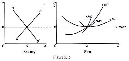
The industry is in long-run equilibrium when a price is reached at which all firms are in equilibrium (producing at the minimum point of their LAC curve and making just normal profits). Under these conditions there is no further entry or exit of firms in the industry, given the technology and factor prices. The long-run equilibrium of the industry is shown in figure 5.15. At the market price, P, the firms produce at their minimum cost, earning just normal profits. The firm is in equilibrium because at the level of output X.

LMC = SMC = P = MR

This equality ensures that the firm maximizes its profit. At the price P the industry is in equilibrium because profits are normal and all costs are covered so that there is no incentive for entry or exit. That the firms earn just normal profit (neither excess profits nor losses) is shown by the equality

LAC = SAC = P

which is observed at the minimum point of the LAC curve. With all firms in the industry being in equilibrium and with no entry or exit, the industry supply remains stable, and, given the market demand (DD’ in figure 5.15), the price P is a long-run equilibrium price.

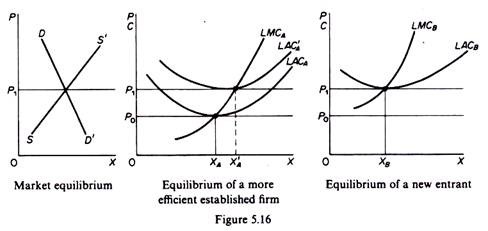
Since the price in the market is unique, this implies that all firms in the industry have the same minimum long-run average cost. This, however, does not mean that all firms are of the same size or have the same efficiency, despite the fact that their LAC is the same in equilibrium. The more efficient firms employ more productive factors of production and/or more able managers.

These more efficient factors must be remunerated for their higher productivity, otherwise they will be bid off by the new entrants in the industry. In other words, as the price rises in the market the more efficient firms earn a rent which they must pay to their superior resources. Thus rents of more efficient factors become costs for the individual firm, and hence the LAC of the more efficient firms shifts upwards as the market price rises, even if the factor prices for the industry as a whole remain constant as the industry expands.

In this situation the LAC of the old, more efficient, firms must be redrawn so as to be tangent at the higher market price. The LMC of the old firms is not affected by the rents accruing to its more productive factors. (It will be shifted only if the prices of factors for the industry in general increase.) Thus the more efficient firms will be in equilibrium, producing that output at which the redrawn LAC is at its minimum (at which point the LAC is cut by the initial LMC given that factor prices remain constant).

Under these conditions, with the superior, more productive resources properly coasted at their opportunity cost, all firms have the same unit cost in their long-run equilibrium. This is shown in figure 5.16. At the initial price P₀ the second firm was not in the industry as it could not cover its costs at that price. However, at the new price, P₁ firm B enters the industry, making just normal profits. The established firm A earns rents which are imputed costs, so that its LAC upwards and it reaches a new ling-run equilibrium a higher level of output (X’ _A).

Optimal resources allocation:

In perfect competition the market mechanism leads to an optimal allocation of resources.

The optimality is shown by the following conditions which prevail in the long-run equilibrium of the industry:

(a)The output is produced at the minimum feasible cost.

(b) Consumers pay the minimum possible price which just covers the marginal cost of the product, that is, price = opportunity cost.

(c) Plants are used at full capacity in the long run, so that there is no waste of re­sources.

(d)Firms only earn normal profits.

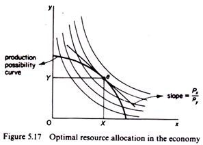
In the long run these conditions prevail in all markets, so that resources are optimally allocated in the economy as a whole. If we assume for simplicity that there are only two commodities (x and y) produced in the economy we may present the allocation of the given resources of the economy with the familiar production-possibility curve. The preferences of the consumers in the economy may be shown by community indifference curves.

Given the production-possibility curve and consumers’ preferences, perfect competition will lead to the optimal allocation of resources under the following con­ditions:

Firstly, if the consumers’ sovereignty, expressed by the price system (uncontrolled by any government intervention), reflects the correct ranking of preferences of the com­munity.

Secondly, if there are no unexhausted economies of scale in any one industry.

Finally, if resources and technology are given; there is no growth in the economy and no technical progress.

If the above conditions are fulfilled, perfect competition leads to the optimal resource allocation defined by the point of tangency of the given production-possibility curve with the highest possible indifference curve. In figure 5.17 optimal allocation of resources is reached at point e. The economy uses up all the available resources (point e lies on the production-possibility curve) and consumers attain the highest possible welfare, given the available factors of production. The optimal allocation is attained at the prices P_x and P_y at which the levels of output of the two commodities are OX and OY.