Income Demand for Labour (With Graph) | Firm

In this article we will discuss about the income demand for labour, explained with the help of a suitable graph. 

The market demand for a commodity at any given price, by definition, is the summation of the individual demands at that price. So the market demand curve for the commodity is the horizontal or lateral summation of the individual demand curves.

The market demand for a variable input, say, labour, at any given rate of wage (W), is also the summation of the labour demand of individual firms at that W. But the market demand curve for labour is not obtained as the horizontal summation of the labour demand curves of the individual firms.

This is because, as W falls and all the firms increase their labour demand, the quantity of output produced would also increase, i.e., the supply of the product at any particular price increases, which means the supply curve of the product shifts to the right, demand condi­tions remaining the same. Consequently, the price of the product falls, causing a leftward shift in the MRP_L = VMP_L curve.

As a result of this, the labour demand curve of the individual firm would shift to left. Since the individual labour demand curves change their position as W changes, the market demand curve for labour cannot be obtained as a horizontal summation of these curves.

It may be noted that in the case of a commodity, as its price falls, and the buyers buy more of the commodity, nothing happens, by virtue of the ceteris paribus assumption, to cause a shift in the individual demand curves. So the market demand curve for a commodity could be obtained as a horizontal summation of the individual demand curves.

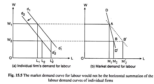
We may explain the process of obtaining the market demand curve for labour with the help of Fig. 15.5. We have shown the labour demand curves of a typical firm in Fig. 15.5(a) and the market demand curve for labour in Fig. 15.5(b).

Let us suppose that, initially, the firm’s labour demand curve is d₁d’₁ and, at the rate of wage W₁, the firm buys L₁ of labour [Fig. 15.5(a)] and all the firms together are buying M, of labour at the point A [Fig. 15.5(b)], Let us now suppose that the rate of wage falls from W₁ to W₂.

If other things, especially the price of the product labour produces, remained the same, then this firm’s and all other firms’ labour demand curves would have remained unchanged and the firm would have bought L’₂ of labour at W = W₂, and the market demand for labour would have been obtained to be, say, M₂ at the point B’.

The market demand curve for labour in this case would have been obtained by joining the points A and B’, and this would have been the horizontal summation of the individual labour demand curves like d₁d’₁ in Fig. 15.5(a).

But as we have seen, the other things do not remain the same. As W falls, and the firms use more of labour, the supply curve of the product would shift to the right and the price of the product would fall. As a result, the firms’ labour demand curves would shift to the left. In Fig. 15.5(a), the individual labour demand curve would shift from d₁d₁ to, say, d₂d₂.

So now at W = W₂, the labour demand of the firm would be L₂, and it would be less than L₂. At W = W₂, the market demand for labour would not be M₂, it would be somewhat less, say M₂, at point B. Therefore, if, we join the points A and B in Fig. 15.5(b), by a curve, we would obtain the market demand curve for labour, DD’, which is steeper than the horizontal summation curve AB’.