Long-Run Equilibrium of the Firm and Industry

In this article we will discuss about the long-run equilibrium of the firm and industry.

Increase and Decrease in the Number of Firms in the Long Run:

We know that the short-run equilibrium of a competitive firm, in the short run, the firm may earn pure profit, i.e., profit in excess of normal profit, as also the profit less than the normal profit, or just the normal profit.

One of the characteristic features of perfect competition is that, here, if the firms earn more than normal profit in the short run, then in the long run, new firms would find it profitable to enter the industry, i.e., in the long run, the number of firms in the industry will increase.

On the other hand, if, in the short run, the firms are not able to earn even the normal profit, i.e., if they suffer losses and if they have no prospect of earning normal profit even in the long run, then no new firm would enter the industry in the long run, rather, the existing firms would be leaving the industry, i.e., the number of firms will decrease in the long run.

Lastly, if the existing firms expect to earn just the amount of normal profit in the long run, then no new firm would enter the industry, nor any existing firm would leave the industry, i.e., the number of firms would not tend to change in the long run.

Increasing Cost, Decreasing Cost and Constant Cost Industries:

As the number of firms in an industry increases, the firms belonging to it may enjoy certain external economies and may also suffer from some external diseconomies. For example, with the increase in their number, the firms may set up a chamber of commerce-like organisation, or, they may establish some research and development (R and D) institute, and all the firms may make use of the beneficial services of these organisations.

As a result, the average cost of the product will diminish, and the LAC curve of each firm will shift downwards. On the other hand, as the number of firms increases, the demand for the inputs also increases and their prices will increase. Consequently, the average cost of the product will increase, and the LAC curve of each firm will shift upwards.

The increasing cost industries are those for which external diseconomies are greater than external economies with the net result that as the number of firms increases (decreases), the LAC curve of each firm shifts upwards (downwards).

On the other hand, the decreasing cost industries are those for which the external economies are greater than external diseconomies with the net result that as the number of firms increases (decreases), the LAC curve of each firm shifts downwards (upwards).

Lastly, for the constant cost industries, the external economies and diseconomies are equal with the result that, as the number of firms increases (decreases), there will be no shift in the LAC curves of the firms.

Assumptions:

To make our analysis of long-run equilibrium of the firm and the industry more simple, we shall make the following (additional) assumptions:

(i) All the firms in the industry are equal in all respects. Therefore, their cost curves are identical.

(ii) If, in the short run, the firms happen to earn less than normal profit, and if they do not see any prospect of earning normal profit or more, even in the long run, then they would be leaving the industry in the long run, but not all at the same time.

For the preparations for leaving the industry to be finished, some firms may require relatively more time than others. Also, the alternative areas of activity may not be the same for all the entrepreneurs. Therefore, the time to leave the industry would be different for different firms.

(iii) The competitive industry under discussion is a constant cost industry. That is, in the long run, external economies and diseconomies that arise from changes in the number of firms, are equal. This assumption implies that in the long run, even when the number of firms changes, the cost curves of each firm would not change their positions—they would remain the same.

From Short-Run Equilibrium to Long-Run Equilibrium:

On the basis of the above assumptions, we shall discuss the long-run equilibrium of a competitive firm. Let us remember that the profit maximising or equilibrium conditions of the competitive firm in the long run are

First order condition: MR = LMC => p = LMC                 (10.27)

Second order condition: d/dq(LMC) > 0                         (10.28)

Cases of Long-Run Equilibrium:

Let us now discuss the long-run equilibrium. There may be three cases.

Case I: The Firms within the Industry are Earning More than Normal Profit in the Short Run.

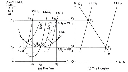
In Fig. 10.7(a), we have shown the short-run and the long-run equilibriums of such a firm. In this Fig. the SAC₁ and SMC₁ curves are the short-run average and marginal curves of the firm in the initial situation, and the LAC and LMC curves are its long-run average and marginal cost curves.

In Fig. 10.7(b), SRS₁ curve is the short-run supply curve of the industry in the initial situation and the D₁D₁ curve is the demand curve for the product of the industry (which is also called the industry’s demand curve), or, the market demand curve for the product.

The price of the product that is determined in the market at the point of intersection, T₁, of these two curves, is p₁. At this price, the AR = MR curve of the firm is AR₁ = MR₁ and its short-run
equilibrium point is the point E₁ in Fig. 10.7(a).

The firm’s short-run supply at this point is q₁, and each firm is earning more than normal profit at E₁(p₁, q₁), since at this point its AR has been greater than SAC. Therefore, by assumption (ii), the number of firms in the industry will be increasing in the long run.

The existing firms also would be increasing their size or scale, and they will be increasing their output thereby to reach the point of intersection E₃ of their MR₁ and LMC curves so that the condition (10.27) may be satisfied—i.e., they would be shifting rightward over time from one SAC curve (or plant curve) to another along their respective LAC curves. As a result, their SMC curves also would be shifting rightward.

Now, in the long run, as the number of firms increases and as the size of the existing firms increases, the SRS curve of the industry would be shifting to the right in Fig. 10.7(b). For, as we know, this curve is the horizontal summation of the firms’ SRS curves.

The demand curve for the product, D₁D₁, remaining the same, the more the SRS curve of the industry shifts to the right, the more the point of intersection of these two curves would move downward towards right along the D₁D₁ curve, and more would be the fall in the price of the product.

Now, as the price diminishes, the AR = MR line of each firm would be shifting downwards and its long-run equilibrium point would be moving from E₃ downward towards left along the firm’s LMC curve to the minimum point E₂(p₂, q₂) of this curve.

In the long run, ultimately, the price of the product would diminish to such a level that the firm’s AR = MR line would shift sufficiently downwards to touch its LAC curve at the latter’s minimum point.

For example, in Fig. 10.7(b), when the SRS curve of the industry (or of the product), while shifting to the right, has come to a position like SRS₂, the price will diminish from p₁ to p₂, the AR = MR line of the firm would shift downwards from AR₁ = MR₁ to AR₂ = MR₂ and it has been a tangent to the firm’s LAC curve at its minimum point E₂.

As we know, the minimum point of the LAC curve lies also on the upward sloping segment of the LMC curve.

Therefore, at this point [E₂(p₂, q₂)], we have the following conditions satisfied:

First, MR = LMC                                  (10.27)

Second, the slope of the horizontal MR curve (= 0) < the slope of the upward sloping LMC curve (= +ve)

i.e., d/dq (LMC) > 0                          (10.28)

Third, AR = LAC                                  (10.29)

⇒ AR x q₂ = LAC X q₂

⇒ TR|_{atq = q2}= LTCl_{at q = q2}           (10.30)

Now, since the conditions (10.27) and (10.28), i.e., the first order and second order conditions of maximum profit have been satisfied, the firm would be able to earn maximum profit at E₂ itself. Therefore, the existing firm will no longer tend to increase its output by increasing its size.

Again, since conditions (10.29) and (10.30) have been satisfied, the firms already existing within the industry will be able to earn only the normal profit. Therefore, the entry of new firms in the industry will stop as soon as the price of the product comes down to p₂.

As a result, the SRS curve of the industry would no longer have a tendency to shift to the right from SRS₂, and the price of the product would not come down further from p₂, and the firm also would not tend to move from the point E₂.

Therefore, E₂ would be the firm’s long-run equilibrium point where, at p = p₂, it would produce and sell an output of q₂ per period and earn only the normal profit. In the above discussion, the minimum point of the firm’s LAC curve is its long-run equilibrium point. This point lies on the firm’s AR = MR, LAC and LMC curves.

Again, since E₂ is the minimum point of the LAC curve, it would also be the minimum point of the firm’s SAC₂ curve (which is the associated SAC curve at that point). Therefore, at the long- run equilibrium point of the firm, we obtain

 

 

 

 

 

 

Since conditions (10.32) and (10.33) have been satisfied the firm would be in short-run equilibrium also at the point E₂ and, owing to (10.34), the firm would earn only the normal profit in this equilibrium.
In our above analysis, therefore, that at the long-run equilibrium point, the firm would simultaneously be in short-run equilibrium, and in this long-run and short-run equilibrium, it would earn only the normal profit.

We may note here that, even after it has reached the point E₂, if the existing firms increase their size and output, and if the new firms still continue to enter the industry, then the SRS curve of the industry would shift to the right of SRS₂, and the price will fall below p₂. If this happens, then each firm would be in a loss-making situation (AR < LAC ⇒ TR < LTC). For, now the whole of the AR curve would go below the LAC curve.

The firms within the industry reach the long-run equilibrium, both entry of new firms in the industry and the process of the size of the industry increasing would come to an end and so the industry also would reach the long-run equilibrium. That is why the long-run equilibrium of the firms also gives us the long-run equilibrium of the industry.

Case II: The Firms are Suffering Irreversible Losses in the Short Run:

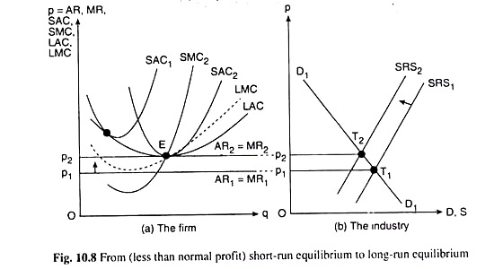
Here we shall discuss a situation where the firms are not able to earn even the normal profit in the short run, neither do they have any prospect of earning at least the normal profit in the long run. Such a situation, depicted in Fig. 10.8, would arise if the price of the product, p₁, is so low that the firm’s AR = MR line throughout its length lies below its LAC and SAC curves.

In this case, in the initial situation, whatever be the firm’s SAC curve the firm’s short-run profit would be less than its normal profit (^._.^. AR < SAC).

Again, since the whole of the AR curve lies below the LAC curve, at any q the firm would have AR < LAC, i.e., whatever output the firm might produce it would earn less than normal profit also in the long run. Therefore, in such a situation, the existing firms would be leaving the industry in the long run.

As the number of firms decreases, the SRS curve of the industry in Fig. 10.8(b) will be shifting to the left. Now, if the demand curve for the product, D₁D₁, remains the same, then the point of intersection of the DD and SRS curve will move upward towards left along the D₁D₁ curve and the price of the product will increase.

Consequently, the AR = MR curve of the firm will be shifting upwards till it touches the LAC curve at its minimum point E (at p = p₂) in Fig. 10.8(a).

At the point E, the conditions (10.27) and (10.28) of the long-run equilibrium of the firm will be satisfied. Therefore, the remaining firms (those who have not yet left the industry) would move to point E by effecting suitable changes in their plant size.

At this point, the firm’s SAC and SMC curves would be SAC₂ and SMC₂ respectively. At the point E(p₂, q₂) the conditions (10.29) and (10.32)-( 10.34) are also satisfied. Therefore, at this point, the firm would be in the short-run and long-run equilibrium—and would earn only the normal profit.

Since all of the remaining firms are now able to earn the normal profit the exodus of firms from the industry and the process of decreasing the plant size of the firms would now stop. Therefore, now, the industry also would be in long-run equilibrium.

Case III: The Firms are Earning Only Normal Profit in the Short Run:

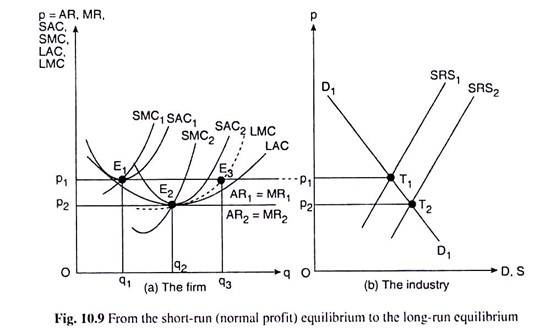
If the existing firms in the industry happen to get only the normal profit in the short run with a prospect to earn pure economic profit in the long run, then there would be no tendency for the new firms to enter the industry or for the existing firms to leave the industry. We shall explain with the help of Fig. 10.9 how the existing firms, in this case, would move from short-run equilibrium to long-run equilibrium.

In Fig. 10.9(a), we have shown the LAC and LMC curves of the firm, and here SAC₁ curve is the firm’s SAC curve in the initial situation. Let us suppose that initially the price of the product that has been determined in the market is p, and at this price the AR₁ = MR₁ curve of the firm has touched its SAC, curve at its minimum point, E₁(p₁, q₁).

At this point the firm produces q, of output per period and sells it at p = p₁, and earns just the normal profit, for, at E₁, the conditions (10.32)—(10.34) have been satisfied.

Now, it is seen clearly in Fig. 10.9 that the firm’s possible long-run equilibrium point is the point of intersection, E₃(p₁, q₃), of the MR and LMC curves, and in order to reach this point, each of the existing firms in the industry would change their scales (sizes) to produce more. Here no new firm would enter the industry because the existing firms are earning no more than the normal profit.

Since the existing firms now would be increasing their scales, the SRS₁ curve of the industry would be shifting to the right. If the demand curve D₁D₁ remains the same, then the price of the product now would diminish along this curve, and, consequently, the firm’s AR = MR line would be shifting downwards till this line, viz., AR₂ = MR₂, touches the LAC curve at its minimum point, E₂(p₂, q₂), in Fig. 10.9 (a):

This would occur when in Fig. 10.9(b), the SRS₁ curve of the industry would shift to SRS₂ and the price of the product would be p₂. At the point E₂ in Fig. 10.9(a), the conditions (10.27)-(10.34) would be satisfied, and so here the firms would reach their short-run and long-run equilibrium points and earn only the normal profit.

If the firms increase their size and their output beyond this situation, the price of the product would fall below p₂, and, consequently, AR = MR curve of each firm would go below the LAC curve and the firm would earn less than normal profit.

That is why no firm would do such thing. Therefore, the point E₂ would be the firm’s long-run (and also short-run) equilibrium point. At the point E₂, the process of increasing the size of the existing firms and that of the industry would stop. So now the industry also would be in long-run equilibrium.