Long Run Supply Curve of the Industry | Perfect Competition

In this article we will discuss about the long run supply curve of the industry under perfect competition.

There are three cases:

(I) The LRS curve of the industry under increasing cost conditions;

(II) The LRS curve of a decreasing cost industry; and

(III) The LRS curve of a constant cost industry.

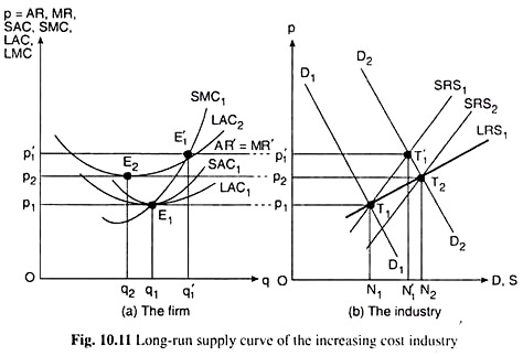
We shall derive the industry’s long run supply curves in the above three cases with the help of Figs. 10.11-10.13. In each of these figures, we have assumed that in the initial situation, the price of the product is p, and at this price, the competitive firm is in short-run as well as in long- run equilibrium at the point E₁ (p₁, q₁), and producing an output of q₁, in part (a) of each of these figures, and so, the industry also is in long-run equilibrium.

E₁ is the minimum point of the LAC₁ and the SAC₁ curves of the firm where the AR₁ = MR₁ line has touched these two curves, and here the firm is earning only normal profit, since we have LAC = SAC = AR = p. Now, in part (b) of each figure, we see that the demand curve for the product, D₁D₁, has intersected the SRS₁ curve of the industry at the point T₁ (p₁, ON₁), to determine the price p₁ of the product.

Therefore, the initial market equilibrium or demand-supply equilibrium point is T₁ where we have obtained the price of the product to be p₁ (or, Op₁) and at this price industry’s short-run and long-run supply, ON₁ = p₁T₁ (which is equal to each firm’s short-run and long-run supply, q₁, multiplied by the number of firms) has been equal to the market demand for the industry’s product.

Since the point T₁ gives us a combination of the price of the product (p₁) and the industry’s long-run equilibrium supply (p₁T₁), T₁ is a point on the SRS₁ curve and also on the long run supply curve of the industry.

Let us now suppose that there is a disturbance in the market in the form of an increase in the demand for the product. As a result, the demand curve shifts to the right from D₁D₁ to, say, D₂D₂ in part (b) of each figure.

Consequently, the initial equilibrium situation is disturbed, for now at price, p₁, demand would be greater than supply. As a result, the price would increase in the short run from p₁ to p’₁ at the new short-run market equilibrium point T’₁ (p’₁, ON’₁).

Now, as price rises in the short run from p₁ to p’₁, the firm’s AR = MR curve shifts upwards from AR₁ = MR₁ to AR’ = MR’ which would intersect the firm’s SMC, curve at the point E’₁ (p’, q’) and the firm’s new short-run equilibrium point would be E’₁ where the firm would produce and sell q’ of output at p = p’.

Since at the short-run equilibrium point E’₁, the firm’s AR > SAC, each firm now would be earning more than normal profit in the short run. Therefore, by assumption, new firms would be joining the industry and the existing firms would be increasing their scales, and a long-run adjustment process would follow.

As the number of firms increases in the long run and the existing firms also increase their output by changing scales of production, the SRS curve of the industry would be shifting to the right, for now, at any particular price, more and more supply would be forthcoming.

As the SRS curve shifts to the right, its point of intersection with the new demand curve, D₂D₂, would be moving downward towards right along the latter curve, and the price of the product would be coming down, and along with this, the AR = MR line of each firm would be shifting downwards.

This is one side, i.e., the revenue side of the process. We have to integrate this with the other side, which is the cost side of process, and arrive at the final long-run equilibrium situation. On the cost side we would have three cases.

1. The Increasing Cost Industry:

Here, as the number of firms increases in the long run, the (envelope) LAC curve of each firm would be shifting upwards (along with its enveloped SAC curves) from the initial LAC) cure. We may see what would happen in this case with the help of Fig. 10.10.

 

In the long-run adjustment process, the firm’s AR = MR line would be shifting downwards from AR’ = MR’ in Fig. 10.11(a), as the price of the product decreases from p’₁ in Fig. 10.11(b).

On the other hand, we have just said, the LAC curve of each firm would be shifting upwards from LAC₁. That is, one curve is shifting downwards from above and the other curve is shifting upwards from below. Therefore, somewhere, in between, the two curves would touch each other.

In Fig. 10.11(a), they have touched each other at the point E₂(p₂, q₂), when p has come down from p₁ to p₂. The price p = p₂ has been determined in the market, i.e., in part (b) of Fig. 10.11, when the SRS curve of the industry has shifted to a position like SRS₂ and intersected the D₂D₂ curve at the point T₂(p₂, ON₂).

At the point E₂, the firms are again in long-run, and also in short-run, equilibrium, since here the AR = MR curve of each firm has touched the LAC curve and also the SAC curve (not shown in the diagram) at their minimum points.

Therefore, at p = p₂, when the supply of each firm is q = q₂ and the supply of the industry is p₂T₂ (or, ON₂), the industry would again be in long-run equilibrium. Therefore, the point T₂(p₂, ON₂) is a point on the LRS curve of the industry.

We have now obtained two points on the long run supply curve of the industry, viz., T₁ and T₂. We may obtain more such points, if we suppose that the demand for the product rises (or falls) again and again. If we join the points T₁, T₂, etc. by a curve in Fig. 10.11(b), we shall obtain the industry’s long run supply curve, viz., LRS₁. This curve gives us that at p = p₁, the industry’s LRS is ON₁ and at p = p₂, the industry’s LRS is ON₂, and so on.

It is clear from Fig. 10.11 (b) that the LRS curve of the industry under increasing cost conditions would be sloping upward towards right. That is, under conditions of increasing cost, the supply of the industry may increase in the long run in response to an increase in demand, but only when price of the product increases. Here the supply increases from ON₁ to ON₂ when price increases from p₁ to p₂.

2. The Decreasing Cost Industry:

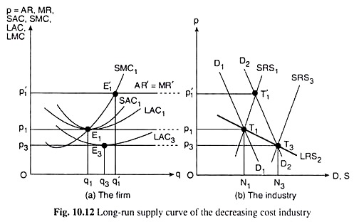
In this case, as the number of firms increases in the long run, the LAC curve of each firm would be shifting downwards from the initial LAC₁ curve. We may see what would happen here with the help of Fig. 10.12.

On the one hand, the firm’s AR = MR line would be shifting downwards from AR’ = MR’ in Fig. 10.12(a), as p decreases from p’₁ in Fig. 10.12(b). On the other hand, the LAC curve of each firm in the decreasing cost industry would be shifting downwards from LAC, in Fig. 10.12(a).

Since, to start with, the AR’ = MR’ curve is above the LAC₁ curve, the former curve in this case would be chasing downwards the latter curve. As the number of firms increases in the long run, and the LAC curve shifts downwards, the profitability of the industry will increase, which will attract more firms to the industry in the long run (than what happened in Case I).

Consequently, in Fig. 10.12(b), the SRS curve would be shifting faster to the right and p would be decreasing faster and the AR = MR curve in Fig. 10.12(a), would also be shifting downwards faster.

The race would come to an end when the AR = MR curve coming downwards more swiftly would touch the downward shifting LAC curve at the point E₃ (p₃, q₃) which is the minimum point of the LAC₃ curve and that of the associated SAC curve (not shown in the figure).

Therefore, each firm would again be in long-run and also in short-run equilibrium at E₃ producing an output of q₃ at the price p₃, and so now the industry would also be in equilibrium. All this happens when the SRS curve has shifted from SRS₁ to the position of SRS₃ and intersected the D₂D₂ curve at the point T₃ (p₃, ON₃) to give us p = p₃.

Therefore, what we have obtained is that, at p = p₃, the firms would be in long-run equilibrium and the industry would also be in long-run equilibrium and at p = p₃, the firm’s supply would be q₃ and the industry’s supply would be p₃T₃ = ON₃. Therefore, the point T₃(p₃, ON₃) in Fig. 10.12(b) would be a point on the industry’s LRS curve.

Therefore, we have obtained two points, T, and T₃, on the long run supply curve of the industry. If we join these two (and more such) points by a curve, we would obtain the LRS curve of the industry under decreasing cost conditions.

It is evident in Fig. 10.12(b) that this LRS curve, viz., LRS₂ would be sloping downward towards right. That is, for a decreasing cost industry, it is possible for the supply of the industry to increase in the long run (here from ON₁ to ON₃) in response to an increase in demand, and that too at a lower price.

3. The Constant Cost Industry:

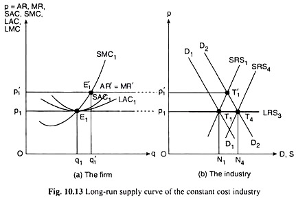
Under conditions of constant cost, as the number of firms increases in the long run, the LAC curve of each firm would not change its position, i.e., it would shift neither upwards nor downwards. On the other hand, the AR = MR curve would be shifting downwards as p decreases owing to rightward shifts in the SRS curve of the industry.

In the long run, the process would come to an end when the AR = MR curve has shifted downwards sufficiently to touch the LAC₁ curve again at the point E₁ (p₁, q₁) in Fig. 10.13(a). The firms and the industry would again be in long- run equilibrium. All this happens when the SRS curve in Fig. 10.13(b) has shifted rightward to the position of SRS₄ and intersected the D₂D₂ curve at the point T₄ (p₁, ON₄) to give us p = p₁.

Now at p = p₁, the firms would be in long-run equilibrium, each producing an output of q, and the industry would also be in long-run equilibrium supplying an amount of ON₄ = p₁T₄. Therefore, the point T₄(p₁, ON₄) would be a point on the industry’s LRS curve.

In the new situation, although each firm produces the initial quantity, q₁, industry’s supply is greater (p₁T₄ being greater than p₁T₁), because, the number of firms now is greater than what it was initially.

We have obtained, therefore, two points, T₁ and T₄, on the industry’s LRS curve. If we join these points by a curve we would obtain the LRS curve of the industry under constant cost conditions. It is seen from Fig. 10.13(b) that this LRS curve, viz., LRS₃, would be a horizontal straight line.

That is, under constant cost conditions, it is possible for the industry to increase its supply in the long run (here from ON₁ to ON₄) in response to an increase in demand, and at the same price.

To conclude, we have seen that the long-run supply (LRS) curve of the industry may be upward sloping, downward sloping, or may be horizontal—depending on whether the industry is increasing cost, decreasing cost or constant cost, i.e., depending on the relative strength of external economies and diseconomies.