Practical Applications of Perfect Competition (With Diagram)

The price determination by the interaction of demand and supply curves has very significant applications in the economic theory.

A few selected cases are discussed below:

I. Shut Down Situations:

Under perfect competition, a firm is a price taker i.e. the price is given to the firm. In the market, the price is determined by the forces of demand and supply.

Given the price the firm can maximize supernormal profits, break even, minimise losses or shut down.

Thus, shut down point occurs when the price is so low that it cannot pay the fixed costs. The losses are incurred and are equal to fixed costs.

The price covers the AVC. There are two shut down situations as:

1. When the firm decides to shut down.

2. When the firm actually shuts down.

1st Case: When the Firm Decides to Shut Down

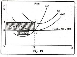
This situation occurs when the price line passes through the minimum point of the AVC curve. It is shown in figure 13. In this diagram, we see that at price OP, equilibrium is at point E where MR = MC. The slope of MC is greater than zero. The firm sells OX units of output.

The loss in this situation is calculated as:

Loss per unit

= Cost per unit – Revenue per unit

= CX – EX = CE

Total Losses

= Loss per unit X Equilibrium Output

= CE X OX

= Shaded Rectangle (ACEP)

= Fixed Costs

Thus the firm decides to shut down at this point.

2nd Case: When the Firm Actually Shuts Down:

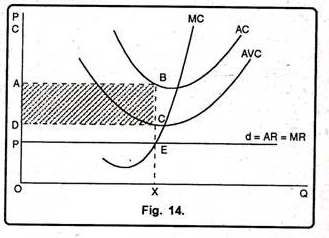
The prices below OP, the firm shuts down as losses are more than the fixed costs. The firms will not be able to cover even AVC. This fact is clear from figure 14.

In figure 14, when price falls to OP, below the shut down point, Equilibrium takes place at point E. Losses which are incurred are equal to BE per point.

Total Losses

= Total Rectangle (ABEP)

= Shaded Rectangle ABCD + rectangle DCEP

= TFC + some part of TVC.

Since, losses are more than TFC, the firm shuts down its unit.

II. Price Controls:

Government often intervenes in the market to control prices. Government through legislation declares that prices in some markets are too high or too low. Price controls can be in the form of either floors or ceilings. These floor or ceiling prices check markets from moving to equilibrium.

1. Price Ceiling:

Consumers convince the government to hold the price of sugar, salt, fuel, houses etc. below the equilibrium price. The Rent Control Act, price ceiling is a law or regulation which holds the market price below the equilibrium level.

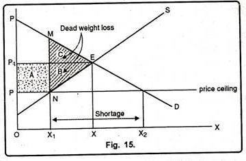
In other words, maximum permissible prices are binding on all. When the price ceilings are imposed, the market disequilibrium leads to inefficiency and black marketing. Figure 15 is the evidence.

In figure 15 price ceiling causes inefficiency.

Let us assume that market for good X is perfectly competitive, where:

E = It is the equilibrium point attained by intersection of demand and supply curves, D and S respectively. P₁ and X are equilibrium price and quantity. Here quantity OX maximises the net social gains.

P = Maximum price or price ceiling imposed on good X. At price P, consumers would like to demand more (X₂) while only X₁ units will be produced.

X₁X₂ = It is the excess demand and shortage in supply. It gives rise to long queues and allocation of limited goods by seller’s preference. it leads to a black market where goods are sold illegally at higher prices.

Considering dead weight loss, it is said that if the production is X₁ units, the net loss of that total surplus or dead weight loss is given by triangle B and C.

This can be calculated as:

Gain in consumer surplus = + (Rectangle A – Triangle C).

Rectangle A is transfer of surplus from producers to consumers. Triangle C is the loss of consumer surplus because consumers can no longer get the supply of X₁X units.

Loss in producer surplus = – (Rectangle A + Triangle B).

Rectangle A, which was producer surplus at price P₁, has gone to consumers as their surplus at price P. Triangle B is the loss in producer surplus at price P.

Therefore, dead weight loss = Net loss of total surplus

= (A – C) + (A – B)

= – C – B= Shaded triangles C and B or ∆MNE.

2. Price Floor:

Generally, businessmen convince the government to hold the price of their products above the equilibrium price. Variety of agriculture policies follows price floor. The Minimum wage Law established a minimum price in the labour market. By adopting this law, the market price will be above the equilibrium level. When price floors are imposed, the market disequilibrium leads to inefficiency.

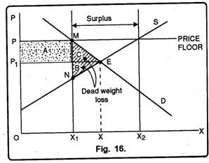
Fig. 16 illustrates that price floor causes inefficiency. Let us assume that the market for good X is perfectly competitive.

Point E = It is the equilibrium point giving P₁ and X as the equilibrium price and quantity which maximizes the net social gains.

P = Minimum price or price floor imposed on good X. At price P, producers would like to produce more (X₂), while only X₁ units will be demanded.

X₁X₂ = It is the surplus supply for which there is no demand.

Considering deadweight loss we see that if the production is according to demand and is only X₁ units, then the net loss of total surplus or deadweight loss is given by triangle C and B. It is calculated as;

Gain in producer surplus = + (Rectangle A – Triangle B).

Rectangle A is transfer of surplus from consumers to producer. Triangle B is the loss of producer’s surplus because the producers are no longer producing X₂X units.

Loss in consumer surplus = – (Rectangle A + Triangle C).

Rectangle A, which was consumer surplus at price Pi, has gone to producers as their surplus at price P. Triangle C is the loss in consumer surplus at price P.

Therefore, deadweight loss = Net loss of total surplus

= (A – B) + (- A – C)

= – B – C

= Shaded triangles B and C or ∆MNE.

From this, we conclude that both price ceilings and price floors are economically inefficient and lead to deadweight loss to the society.

Minimum Support Price and Income Stabilization in Agriculture:

1. Minimum Support Price:

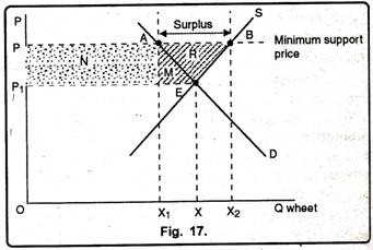
Minimum support price is a government-established minimum price. The government has fixed support prices for a number of agricultural products, such as wheat, rice, etc. The minimum support price holds the market price above its equilibrium level. The effect of imposing the minimum support price for wheat is explained in fig. 17, where

P₁ = In the absence of the price floor, the wheat market is in equilibrium at point E, P₁ is the equilibrium price at which OX units of wheat are demanded and sold.

P = It is the support price which is above the equilibrium price, P₁. This price is called a support price because when it is necessary, the government decides to support the price at P. At this price, farmers would like to supply X₂ units of wheat while only X₁ units will be demanded.

X₁X₂ = It is surplus wheat.

Cost to the government = The entire surplus of X₁X₂ is purchased by the government from the farmers at price P. The cost to the government is equal to X₁ AB X₂.

Gain to the producers = Farmers are selling X₂ units of wheat at price P and are enjoying a surplus of rectangle N + triangle M + triangle R.

Loss to the consumers = At legal price P, consumers lose their surplus shown by the Rectangle N which goes to producers and triangle M which is deadweight loss.

The total loss of consumer surplus = rectangle N + triangle M.

Effects of Minimum Support Price:

1. Farmers benefit because they receive higher price for their product.

2. Farmers’ income rises. Earlier (in equilibrium), the income was OP₁EX. After the minimum support price the income has risen to OPBX_2.

3. Consumers are worse off because they have to pay higher price (P) for wheat under the support price scheme. Loss in consumer surplus = N + M shaded areas.

4. Consumers have to pay higher tax to provide funds to the government for the purchase of surplus wheat. Also, consumers must provide the funds to store and dispose of the surplus.

5. The policy imposes a cost to the government equal to X₁ABX₂.

6. The Food Corporation of India (FCI) procures surplus wheat and rice on behalf of the government. The grain is stored in its warehouses. The government incurs heavy losses as it has to subsidies the consumption of these grains through public distribution system (PDS).

In this way, the policy of minimum support price leads to welfare loss of the society. If the government wants to provide income support to those farmers who are financially distressed and do not have sufficient income to finance their indebtedness, it is better to give them this income directly.

2. Income Stabilisation:

The government can stabilize the income of the farmer’s by allowing changes in price exactly in equal proportion to the changes in production. For example, if production rises by 5% the government should allow only 5% fall in price and vice-versa.

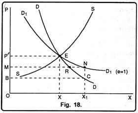
Figure 18 shows how the income stabilisation policy can be pursued efficiently by the government.

Where:

Point E = Equilibrium point where demand (D) and supply (S) curves intersect, giving the market price as OP’ and production as OX.

D₁D₁ = It is the unitary elastic demand curve drawn through point E. On this demand curve, the income earned by the farmer remains constant and is equal to the area of the rectangle OP EX.

OX1 = Assume that actual production is more than OX, say OX₁. In the market system, OX₁ units of output will be demanded at price OB (and not OM). The income earned by the farmer equals area of the rectangle OBCX₁.

Effects of Income Stabilisation Policy are given as:

1. If the government pursues the income stabilisation policy by which it wants to stabilize the farmer’s income at OP’EX then it will not allow the price to fall below OM for OX] level of output. In other words, in the market system price for OX₁ Level of output will be OB and with government’s policy price will be OM. The income earned with price OM is equal to OMNX₁ which is equal to OP’EX. Consumers will buy MR units and RN will be bought by the government.

2. Incomes of the farmers will be stabilised at OP’EX.

Effects of minimum wage law:

Minimum wage law allows the government to fix the minimum wage for certain industries through legislation, to protect the workers against the exploitation of employers. This law has been adopted worldwide. It is particularly relevant for unskilled labour, as this type gets the lowest wage rate. The aim of Minimum Wage Law is to promote equitable distribution of income. In India, the Minimum Wages Act was passed in 1948 and has been revised many times since then.

The minimum wage should be fixed at a level which exceeds the existing equilibrium wage. To analyze the effects of minimum wage, it is assumed that there exists perfect competition among the employers in the industry. The government fixes the minimum wage for this industry.

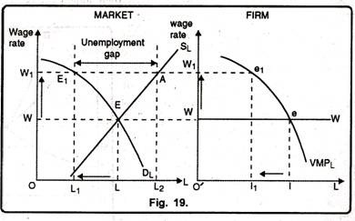
In the perfectly competitive labour market (as shown in the first panel of Fig. 19), the market demand for labour, Dl is the aggregate of the VMP₁ (Value of Marginal Productivity of Labour) curve. The market supply curve, S₁ is upward sloping.

The equilibrium takes place at point E where D₁ = S₁– Equilibrium wage rate is OW and employment level is OL. This is the maximum wage earned by the labour given the profit maximising behaviour of the firms. At this wage rate O’W, the firm is in equilibrium at point e where W = VMP₁ and it employs 01 laborers as shown in the second panel of figure 19.

Now let us assume that the government fixes the minimum wage level at W₁. At the legal minimum wage W₁, market demand would be OL₁ and supply, OL₂. The unemployment gap is L₁, L₂. This unemployment gap can be divided into two parts.

(i) L₁L = they are those workers who have lost the job after the minimum wage fixation but were employed at the earlier wage, OW

(ii) LL₂ = They are those workers who are offering their services at the legal minimum wage W₁, but they are unemployed as there is no demand for them.

The firm also shows reduction in the number of workers employed from OI to OI₁. The effect of the rise in wage rate is to produce unemployment. The workers who lose jobs are worse off. The extent of unemployment depends upon the elasticity of the VMP_L curve. If the VMP₁ curve is inelastic, then unemployment would be much lesser and vice versa.

Solutions to the Problem of Unemployment Caused by Minimum Wage Law:

1. It is possible to pass on the burden of higher minimum wages to the consumers in the form of higher prices. A rise in the price of the product (P_x) will shift the VMP_L curve rightwards (because VMP_L = MP_L X P_X. The result would be lesser unemployment when the legal minimum wage rate (W₁) is imposed as seen in figure 20.

 

When the minimum wage rate W₁ is imposed, unemployment is to the extent of l₁ 1. If the firm raises the price of the product, then the VMP_L curve shifts rightwards to VMP_L7 1 and unemployment is reduced by I₂1.

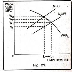
2. If labour markets are characterized by monopoly, it is possible to increase employment. It is shown in Fig. 21.

The monopsonist is in equilibrium at point E where VMP_L = MFC. He employs OL units of labour at wage rate OW per unit. This is the initial position. The value of marginal product of labour at OL level of employment is OW₃. The extent of monopsonistic exploitation is WW₃.

If the Minimum Wage Law fixes the minimum wage at W₃, then employment level remains at OL and wage rate rises to OW₃. If the legal wage is fixed at W₂, then employment level increases and is equal to W₂L₂. If legal wage is W₁, employment level is maximum and is equal to OL₁.

Thus, if there is monopsony in the labour market, the effect of Minimum Wage Law may be to increase employment. This law is particularly useful for low paid workers. With higher wages and income, the productive efficiency of these low-paid workers will improve.

To be more effective, the law should cover all workers. If all the workers are not covered by law, then the one unemployed in the covered sector will shift to the uncovered sector and get employment there.