Supply of Labour (With Diagram) | Employment

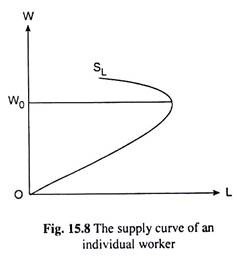
In this article we will discuss about the supply of labour of an individual worker with overtime payment, explained with the help of suitable diagrams.

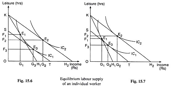
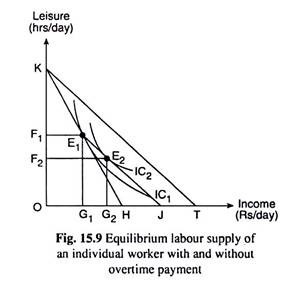
In modern days, union-management contracts provide for extra pay, generally at a higher (than the prevailing) rate for overtime work. Here by overtime work, we would mean any work in excess of what the worker has decided willingly to perform on the basis of his preference-indifference pattern and the given wage rate, W. Let us suppose that initially the worker’s budget line is KH in Fig. 15.9 (like KH) in Fig. 15.6 or 15.7).

Here, if the worker does not work at all and enjoys all the 24 (OK) hours in a day as leisure then he would have zero of income and OK hrs. of leisure at the point K on the vertical axis. On the other hand, if the worker works all the 24 (OK) hrs. and keeps zero hrs. of leisure for himself, then he would have an income of OH (Rs) which is equal to OK x W or 24 x W and the value of which depends upon the value of W.

Now, if we join the points K (0, OK) and H (OH, 0) by a straight line, we would obtain the line KH as the budget line of the worker who may select any income-leisure or income-work combination on the line as he wishes. As we already know, and as we get here also, the rate of wage (per hour) is W = OH/OK which is equal to the reciprocal of the numerical slope of the budget line KH.

Now, given the budget line KH, the worker is in equilibrium at the point E₁ where his indifference curve, IC₁, has been touched by the budget line. At the point E₁, the worker decides to work for KF₁ hrs. and have an income of OG₁ (Rs) per day, his amount of leisure at this point being OF₁ hrs. per day.

Let us now suppose that the overtime wage is twice as much as the ‘regular’ wage rate (W). Therefore, at the overtime wage rate, the worker would have earned OT (= 2.0H) of income if he worked all the 24 hrs. at this rate and then his budget line would have been KT for which the reciprocal of the numerical slope is twice as much as that of the line KH, and the numerical slope is 1/2 of that of the line KH.

In Fig. 15.9, we have drawn E₁J parallel to the line KT. Since the reciprocal of the numerical slope of E₁J is equal to that of the line KT and, therefore, would represent the overtime wage, the budget line of the worker would become E₁J if overtime wage is offered to him at the point E₁.

In other words, if an overtime wage is introduced and the worker decides to work overtime in excess of his normal hours (i.e., KF₁ in this case), then his budget line would be KE₁J in place of KH—the budget line now would have a kink at the point E₁ indicating that its numerical slope in the segment E₁J would be less than (here half of) what it had been in the segment KE₁.

Now, if the budget line of the worker is KE₁J then he would be in satisfaction-maximising equi­librium at the point E₂ on the E₁J segment of the budget line where the line has been a tangent to one of his ICs, viz., IC₂, which is higher than IQ. At the point E₂, the worker now would work for longer hours KF₂ (KF₂ > KF₁) and earn a higher amount of income OG₂ (OG₂ > OG₁), and, consequently, his leisure hours would de­cline from OF₁ to OF₂.

Now, not only the particular worker in Fig. 15.9 but workers, in general, will always supply more hours of labour when they are offered overtime. The reason can be given again in terms of indifference curve analysis. In Fig. 15.9, the consumer is in equilibrium, initially at the point E₁, that is, before the introduction of the wage scheme for overtime work.

E₁ being the point of tangency between the IC, curve and the budget line KH, the consumer’s MRS of income for leisure is equal to the market price of income in terms of leisure. But when the wage scheme for overtime work is introduced, the worker’s budget line be­comes KE₁J, with a kink at the point E₁.

Consequently, at the point E₁, the numerical slope of the IC₁ curve becomes larger than that of the E₁J segment of the budget line, i.e., the MRS of income for leisure becomes larger than the market price of income in terms of leisure.

Therefore, the consumer can no longer be in equilibrium at the point E₁. He would now be moving downward towards right along the E₁J segment of the budget line having more and more of income, i.e., supplying more and more of labour, and taking less and less of leisure till he reaches the point of tangency E₂ between the IC₂ curve—a higher curve than IC₁—and the line E₁J.

At the point E₂, the worker would again reach equilibrium, for now, his MRS of income for leisure has again been equal to the market price of income in terms of leisure. It should be noted here that if overtime were paid before KF₁ hours were worked, the hours of work would not necessarily increase.

Then the kink would lie on the E₁K segment of the initial budget line and the tangency to the highest indifference curve might occur to the left of E₁ reducing the hours of work.