The Phillips Curve: Relation between Unemployment and Inflation

In this article we will discuss about the Phillips curve to study the relationship between unemployment and inflation.

The Phillips curve examines the relationship between the rate of unemployment and the rate of money wage changes. Known after the British economist A.W. Phillips who first identified it, it ex­presses an inverse relationship between the rate of unemployment and the rate of increase in money wages. Basing his analysis on data for the United Kingdom, Phillips derived the empirical relationship that when unemployment is high, the rate of increase in money wage rates is low.

This is because “workers are reluctant to offer their services at less than the prevailing rates when the demand for labour is low and unemployment is high so that wage rates fall very slowly.” On the other hand, when unemployment is low, the rate of increase in money wage rates is high. This is because, “when the demand for labour is high and there are very few unemployed we should expect employer to bid wage rates up quite rapidly.”

The second factor which influences this inverse relationship between money wage rate and unemployment is the nature of business activity. In a period of rising business activity when unemploy­ment falls with increasing demand for labour, the employers will bid up wages. Conversely, in a period of falling business activity when demand for labour is decreasing and unemployment is rising, employ­ers will be reluctant to grant wage increases.

Rather, they will reduce wages. But workers and unions will be reluctant to accept wage cuts during such periods. Consequently, employers are forced to dismiss workers, thereby leading to high rates of unemployment. Thus when the labour market is depressed, a small reduction in wages would lead to large increase in unemployment.

Phillips concluded on the basis of the above argu­ments that the relation between rates of unem­ployment and a change of money wages would be highly non-linear when shown on a diagram. Such a curve is called the Phillips curve.

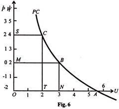
The PC curve in Figure 6 is the Phillips curve which relates percentage change in money wage rate (W) on the vertical axis with the rate of unemployment (U) on the horizontal axis. The curve is convex to the origin which shows that the percentage change in money wages rises with decrease in the employment rate. In the figure, when the money wage rate is 2 per cent, the unemployment rate is 3 per cent.

But when the wage rate is high at 4 per cent, the unemployment rate is low at 2 per cent. Thus there is a trade-off between the rate of change in money wage and the rate of unemployment. This means that when the wage rate is high the unemployment rate is low and vice versa.

The original Phillips curve was an observed statistical relation which was explained theoretically by Lipsey as resulting from the behaviour of labour market in disequilibrium through excess demand.

Several economists have extended the Phillips analysis to the trade-off between the rate of unem­ployment and the rate of change in the level of prices or inflation rate by assuming that prices would change whenever wages rose more rapidly than labour productivity. If the rate of increase in money wage rates is higher than the growth rate of labour productivity, prices will rise and vice versa. But prices do not rise if labour productivity increases at the same rate as money wage rates rise.

This trade-off between the inflation rate and unemployment rate is explained in Figure 6 where the inflation rate (ṗ) is taken along with the rate of change in money wages(ẇ). Suppose labour productivity rises by 2 per cent per year and if money wages also increase by 2 per cent, the price level would remain constant. Thus point B on the PC curve corresponding to percentage change in money wages (M) and unemployment rate of 3 per cent (N) equals zero (O) per cent inflation rate (ṗ) on the vertical axis.

Now assume that the economy is operating at point B. If now, aggregate demand is increased, this lowers the unemployment rate to 07(2%) and raises the wage rate to OS (4%) per year. If labour productivity continues to grow at 2 per cent per annum, the price level will also rise at the rate of 2 per cent per annum at OS in the figure. The economy operates at point C. With the movement of the economy from B to C, unemployment falls to T (2%). If points B and C are connected, they trace out a Phillips curve PC.

Thus a money wage rate increase which is in excess of labour productivity leads to inflation. To keep wage increase to the level of labour productivity (OM) in order to avoid inflation, ON rate of unemployment will have to be tolerated.

The shape of the PC curve further suggests that when the unemployment rate is less than 5½ per cent (that is, to the left of point A), the demand for labour is more than the supply and this tends to increase money wage rates. On the other hand, when the unemployment rate is more than 5½ per cent (to the right of point A), the supply of labour is more than the demand which tends to lower wage rates. The implication is that the wage rates will be stable at the unemployment rate OA which is equal to 5½ per cent per annum.

It is to be noted that PC is the “conventional” or original downward sloping Phillips curve which shows a stable and inverse relation between the rate of unemployment and the rate of change in wages.

Friedman’s View: The Long-Run Phillips Curve:

Economists have criticised and in certain cases modified the Phillips curve. They argue that the Phillips curve relates to the short run and it does not remain stable. It shifts with changes in expectations of inflation. In the long run, there is no trade-off between inflation and employment. These views have been expounded by Friedman and Phelps” in what has come to be known as the “accelerationist” or the “adaptive expectations” hypothesis.

According to Friedman, there is no need to assume a stable downward sloping Phillips curve to explain the trade-off between inflation and unemployment. In fact, this relation is a short-run phenom­enon. But there are certain variables which cause the Phillips curve to shift over time and the most important of them is the expected rate of inflation.

So long as there is discrepancy between the expected rate and the actual rate of inflation, the downward sloping Phillips curve will be found. But when this discrepancy is removed over the long run, the Phillips curve becomes vertical.

In order to explain this, Friedman introduces the concept of the natural rate of unemployment. In represents the rate of unemployment at which the economy normally settles because of its structural imperfections. It is the unemployment rate below which the inflation rate increases, and above which the inflation rate decreases. At this rate, there is neither a tendency for the inflation rate to increase or decrease.

Thus the natural rate of unemployment is defined as the rate of unemployment at which the actual rate of inflation equals the expected rate of inflation. It is thus an equilibrium rate of unemploy­ment towards which the economy moves in the long run. In the long run, the Phillips curve is a vertical line at the natural rate of unemployment.

This natural or equilibrium unemployment rate is not fixed for all times. Rather, it is determined by a number of structural characteristics of the labour and commodity markets within the economy. These may be minimum wage laws, inadequate employment information, deficiencies in manpower training, costs of labour mobility, and other market imperfections. But what causes the Phillips curve to shift over time is the expected rate of inflation.

This refers to the extent the labour correctly forecasts inflation and can adjust wages to the forecast. Suppose the economy is experiencing a mild rate of inflation of 2 per cent and a natural rate of unemployment (N) of 2 per cent. At point A on the short-run Phillips curve SPC₁ in Figure 7, people expect this rate of inflation to continue in the future. Now assume that the government adopts a monetary-fiscal programme to raise aggregate demand in order to lower unemployment from 3 to 2 per cent.

The increase in aggregate demand will raise the rate of inflation to 4 per cent consistent with the unemployment rate of 2 per cent. When the actual inflation rate (4 per cent) is greater than the expected inflation rate (2 per cent), the economy moves from point A to B along the SPC₁ curve, and the unemployment rate temporarily falls to 2 per cent. This is achieved because the labour has been deceived.

It expected the inflation rate of 2 per cent and based their wage demands on this rate. But the workers eventually begin to realise that the actual rate of inflation is 4 per cent which now becomes their expected rate of inflation. Once this happens the short-run Phillips curve SPC₁ shifts to the right to SPC₂. Now workers demand increase in money wages to meet the higher expected rate of inflation of 4 per cent.

They demand higher wages because they consider the present money wages to be inadequate in real terms. In other words, they want to keep up with higher prices and to eliminate fall in real wages. As a result, real labour costs will rise, firms will discharge workers and unemployment will rise from B (2%) to C (3%) with the shifting of the SPC₁ curve to SPC₂. At point C, the natural rate of unemployment is re-established at a higher rate of both the actual and expected inflation (4%).

If the government is determined to maintain the level of unemployment at 2 per cent, it can do so only at the cost of higher rates of inflation. From point C, unemployment once again can be reduced to 2 per cent via increase in aggregate demand along the SCP₂ curve until we arrive at point D. With 2 per cent unemployment and 6 per cent inflation at point D, the expected rate of inflation for workers is 4 per cent.

As soon as they adjust their expectations to the new situation of 6 per cent inflation, the short-run Phillips curve shifts up again to SPC₃ and the unemployment will rise back to its natural level of 3 per cent at point E. If points A, C and E are connected, they trace out a vertical long-run Phillips curve LPC at the natural rate of unemployment.

On this curve, there is no trade-off between unemployment and inflation. Rather, any one of several rates of inflation at points A, C and E is compatible with the natural unemployment rate of 3 per cent.

Any reduction in unemployment rate below its natural rate will be associated with an accelerating and ultimately ex­plosive inflation. But this is only possible temporarily so long as workers overestimate or underestimate the inflation rate. In the long-run, the economy is bound to establish at the natural unemployment rate.

There is, therefore, no trade-off between unemploy­ment and inflation except in the short run. This is because inflationary expectations are revised according to what has happened to inflation in the past.

So when the actual rate of inflation, say, rises to 4 per cent in Figure 7, workers continue to expect 2 per cent inflation for a while and only in the long run they revise their expectations upwards towards 4 per cent. Since they adapt themselves to the expectations, it is called the adaptive expections hypothesis.

According to this hypothesis, the expected rate of inflation always lags behind the actual rate. But if the actual rate remains constant the expected rate would ultimately become equal to it. This leads to the conclusion that a short run trade-off exists between unemployment and inflation, but there is no long run trade-off between the two unless a continuously rising inflation rate is tolerated.

Its Criticisms:

The accelerationist hypothesis of Friedman has been criticised on the following grounds:

1. The vertical long-run Phillips curve relates to the steady rate of inflation. But this is not a correct view because the economy is always passing through a series of disequilibrium positions with little tendency to approach a steady state. In such a situation, expectations may be disappointed year after year.

2. Friedman does not give a new theory of how expectations are formed that would be free from theoretical and statistical bias. This makes his position unclear.

3. The vertical long-run Phillips curve implies that all expectations are satisfied and that people correctly anticipate the future inflation rates. Critics point out that people do not anticipate inflation rates correctly, particularly when some prices are almost certain to rise faster than others. There are bound to be disequilibria between supply and demand caused by uncertainty about the future and that is bound to increase the rate of unemployment. Far from curing unemployment, a dose of inflation is likely to make it worse.

4. In one of his writings Friedman himself accepts the possibility that the long-run Phillips curve might not just be vertical, but could be positively sloped with increasing doses of inflation leading to increasing unemployment.

5. Some economists have argued that wage rates have not increased at a high rate of unemploy­ment.

6. It is believed that workers have a money illusion. They are more concerned with the increase in their money wage rates than real wage rates.

7. Some economists regard the natural rate of unemployment as a mere abstraction because Friedman has not tried to define it in concrete terms.

8. Saul Hyman has estimated that the long-run Phillips curve is not vertical but is negatively sloped. According to Hyman, the unemployment rate can be permanently reduced if we are prepared to accept an increase in inflation rate.

Tobin’s View:

James Tobin in his presidential address before the American Economic Association in 1971 proposed a compromise between the negatively sloping and the vertical Phillips curve. Tobin believes that there is a Phillips curve within limits. But as the economy expands and employment grows, the curve becomes even more fragile and vanishes until it be­comes vertical at some critically low rate of unemploy­ment.

Thus Tobin’s Phillips curve is kinked-shaped, a part like a normal Phillips curve and the rest vertical, as shown in Figure 8. In the figure, Uc is the critical rate of unem­ployment at which the Phillips curve becomes vertical where there is no trade-off between unemployment and inflation. According to Tobin, the vertical portion of the curve is not due to increase in the demand for more wages but emerges from imperfections of the labour market.

At the Uc level, it is not possible to provide more employment because the job seekers have wrong skills or wrong age or sex or are in the wrong place. Regarding the normal portion of the Phillips curve which is negatively sloping, wages are sticky down­ward because labourers resist a decline in their relative wages. For Tobin, there is a wage-change floor in excess supply situations.

In the range of relatively high unemployment to the right of Uc in the figure, as aggregate demand and inflation increase and involuntary unemployment is reduced, wage-floor markets gradually diminish. When all sectors of the labour market are above the wage floor, the level of critically low rate of unemployment Uc is reached.

Solow’s View:

Like Tobin, Robert Solow does not believe that the Phillips curve is vertical at all rates of inflation. According to him, the curve is vertical at positive rates of inflation and is horizontal at negative rates of infla­tion, as shown in Figure 9. The basis of the Phillips curve LPC of the figure is that wages are sticky downward even in the face of heavy unemployment or deflation.

But at a par­ticular level of unemployment when the demand for labour increases, wages rise in the face of expected inflation. But since the Phillips curve LPC becomes vertical at that mini­mum level of unemployment, there is no trade-off between unemployment and inflation.

Conclusion:

The vertical Phillips curve has been ac­cepted by the majority of economists. They agree that at un­employment rate of about 4 per cent, the Phillips curve be­comes vertical and the trade-off between unemployment and inflation disappears. It is impossible to reduce unemployment below this level because of market imperfections.

Policy Implications of the Phillips Curve:

The Phillips curve has important policy implications. It suggests the extent to which monetary and fiscal policies can be used to control inflation without high levels of unemployment. In other words, it provides a guideline to the authorities about the rate of inflation which can be tolerated with a given level of unemployment. For this purpose, it is important to know the exact position of the Phillips curve.

While explaining the natural rate of unemployment, Friedman pointed out that the only scope of public policy in influencing the level of unemployment lies in the short run in keeping with the position of the Phillips curve. He ruled out the possibility of influencing the long-run rate of unemployment because of the vertical Phillips curve.

According to him, the trade-off between unemployment and inflation does not exist and has never existed. However rapid the inflation might be, unemployment always tends to fall back to its natural rate which is not some irreducible minimum of unemployment. It can be lowered by removing obstacles in the labour market by reducing frictions.

Therefore, public policy should improve the insti­tutional structure to make the labour market responsive to changing patterns of demand. Moreover, some level of unemployment must be accepted as natural because of the existence of large number of part-time workers, unemployment compensation and other institutional factors.

Another implication is that unemployment is not a fitting aim for monetary expansion, according to Friedman. Therefore, employment above the natural rate can be reached at the cost of accelerating inflation, if monetary policy is adopted. In his words, “A little inflation will provide a boost at first—like a small dose of a drug for a new addict—but then it takes more and more inflation to provide the boost, just it takes a bigger and bigger dose of a drug to give a hardened addict a high.”

Thus if the government wants to have a genuine full employment level at the natural rate, it must not use monetary policy to remove institutional restraints, restrictive practices, barriers to mobility, trade union coercion and similar obstacles to both the workers and the employers.

But economists do not agree with Friedman. They suggest that it is possible to reduce the natural rate of unemployment through labour market policies, whereby labour market can be made more efficient. So the natural rate of unemployment can be reduced by shifting the long-run vertical Phillips curve to the left.

Johnson doubts about the applicability of the Phillips curve to the formulation of economic policy on two grounds. “On the one hand, the curve represents only a statistical description of the mechanics of adjustment in the labour market, resting on a simple model of economic dynamics with little general and well-tested monetary theory behind it. On the other hand, it describes the behaviour of the labour market in a combination of periods of economic fluctuation and varying rates of inflation, conditions which presumably influenced the behaviour of the labour market itself, so that it may reasonably be doubted whether the curve would continue to hold its shape if an attempt were made by economic policy to pin the economy down to a point on it.”