In valuation of investments, one has to consider his assets in the portfolio as a part of his total investments. In considering the portfolio, not only returns are to be considered as in the case of single investments but their risks also. Two plus two will not make it four in the aggregation of risks, as shown by famous author Markowitz. So the risks in a portfolio of assets will not be the total of individual risks of investments, made; it can be more or less than the total. The objective of investor is to minimise the risk for a given return and capital market theory deals with that subject.
Capital market theory is an extension of the portfolio theory of Markowitz. The portfolio theory explains how rational investors should build efficient portfolio based on their risk-return preferences. Capital Market Asset Pricing Model (CAPM) incorporates a relationship, explaining how assets should be priced in the capital market.
As Betas differ according to the market proxy, that they are measured against, then in effect, CAPM, has not been and cannot be tested. We may recall that CAPM states that-
Return = Risk free rate + Beta (Market Return – Risk free rate)
ADVERTISEMENTS:
A security with a zero Beta should give a risk free return. In actual results these zero beta returns are higher than the risk free return indicating that there are some non-Beta risk factors or some left over unsystematic risk.
Besides, although, in the long-run, high Beta portfolios have provided larger returns than low-risk ones, in the short-run, CAPM Theory and the empirical evidence diverge strikingly and sometimes the relationship between risk and return may turn out to be negative which is contrary to CAPM Theory.
It can thus be concluded that CAPM Theory is a neat Theoretical exposition. The CML and SML are the lines reflecting the total risk and systematic risk elements in the portfolio analysis, respectively. But in actual world, the CAPM is not in conformity with the real world risk-return trends and empirical results have not always supported the Theory atleast in the short-run.
Assumptions of Capital Market Theory:
(1) Investors are expected to make decisions based solely on risk-return assessments (expected returns and standard deviation measures).
ADVERTISEMENTS:
(2) The purchase and sale transactions can be undertaken in infinitely divisible units.
(3) Investors can sell short any number of shares without limit.
(4) There is perfect competition and no single investor can influence prices, with no transactions costs, involved.
(5) Personal income taxation is assumed to be zero.
ADVERTISEMENTS:
(6) Investors can borrow/lend, the desired amount at riskless rates.
Efficient Frontier:
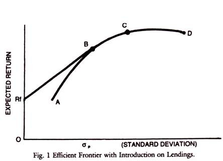
The above assumptions, although some of them are unrealistic provide a basis for an efficient frontier line common to all. Different expectations lead to different frontier lines. If borrowing and lending is introduced the efficient frontier line can be thought of as a straight line. Lending is like investing in a riskless security say of Rf in the Fig.1.
Rf = Risk free investment. If he places part of his funds in Risk free assets (Rf) and part of his funds in risky securities (B) along the efficient frontier, he would generate portfolios along the straight line segment RfB.
Rp = XRm + (1 – x) Rf
where, Rp = expected return on portfolio
X = percentage of funds invested in risky portfolio
(1 – x) = percentage of funds invested in riskless asset
Rm = expected return on risky portfolio
ADVERTISEMENTS:
Rf = expected return on riskless asset
and σp = x σm
σp = expected standard deviation of the portfolio
σM = expected standard deviation on risky portfolio
ADVERTISEMENTS:
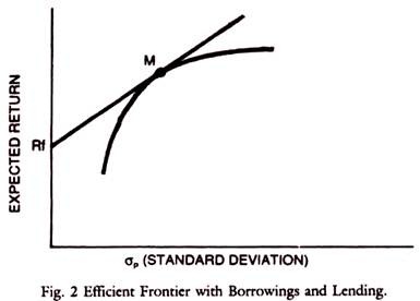
Introduction of both borrowing and lending has given us an efficient frontier that is a straight line throughout as shown in the Fig. 2. M is the optimal portfolio of risky investments. The decision to purchase at M is the investment decision and the decision to buy some riskless asset (lend) or to borrow (leverage the portfolio) is the financing decision.
Capital Market Line:
If all the investors hold the same risky portfolio, then in equilibrium, it must be the market portfolio. In that sense RfM straight line is the Capital Market Line (CML). All investors choose along this line and efficient portfolios will be on this line. Those which are not efficient will however be below the line.
The equation of the capital market line connecting the riskless asset with a risky portfolio is-
ADVERTISEMENTS:
Subscript (e) denotes the efficient portfolio. Rm – Rf/σm can be thought as the extra return that can be gained by increasing the amount of risk on an efficient portfolio by one unit.
Thus,
can be taken to represent the market price of risk times the amount of risk in the portfolio. Rf is the risk-free return for abstaining consumption for period one. Thus, Rf is the price of time or waiting, σe is risk on the portfolio.
Security Market Line:
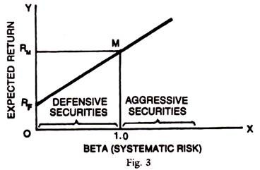
In case of portfolios involving complete diversification, where the unsystematic risk tends to zero, there is only systematic risk measured by Beta (β) the only dimension of a security, which concerns us are expected return and Beta. All portfolios of investments lie along a straight line in the return to Beta space. To determine this line we need to connect the Intercept (where Beta is zero as it is riskless security), and the market portfolio (Beta of one and return of RM).
ADVERTISEMENTS:
These points are Rf and M in the graph below. The equation of that straight line is Security Market Line (SML):
Ri = α + b βi
RF = α as b βi becomes zero for riskless asset (β = 0)
where, β = 1
RM = α + b (1) or RM – α = b
ADVERTISEMENTS:
Since RF = α, then RM – RF = b
Combining the above two results, we have-
Ri = RF + (RM – RF)
This is the key equation for Security Market Line and can be rewritten as Ri – RF = βi (RM – RF)
Market Efficiency and CAPM:
The theory of Market Efficiency and Random Walk Theory explain the price formation through the absorption of information in a perfect manner and postulate that prices move in a random fashion independent of past trends. The market is said to be efficient, if price is determined by competitive forces of supply and demand based on the free flow of correct and full information.
In the real world, information is not free and complete. There are trends in which prices move and technical analysis is the answer and the Dow Theory is applicable here. If the market absorption and information flows are not perfect, market prices move around the intrinsic worth of the shares but may not reach them.
ADVERTISEMENTS:
The actual pricing of shares is to be evaluated in terms of its earnings potential (EPS), dividend distribution, P/E ratio and a host of other financial ratios and a forecast of the prices is to be made to assess whether the share is overpriced or underpriced. Then the principle of buying underpriced shares and selling overpriced shares is adopted by the investor. If the random walk theory is disproved, then the markets are not efficient. CAPM depends on the assumptions of market efficiency, competition and free play of forces in the market.
According to the capital assets pricing model, there is an efficiency frontier for each investor and following the Markowitz model, the capital market line and efficiency frontier line can be drawn to arrive at an efficient portfolio for each investor. The efficient portfolio minimises the risk for a given level of return or maximises the return for a given level of risk. The risk-return analysis under portfolio theory helps the construction of an efficient portfolio.
In modern portfolio theory, the risk is represented by the concept of Beta in substitution of the standard deviation of expected returns in CAPM. This Beta relates the specific risk of a company to market risk and is represented by the slope of the capital market line. The scrips with a high Beta are aggressive such as TELCO and Reliance. They are more risky and give a higher return than the market average. The scrips with a low Beta are defensive and have lower returns but are less risky than the market average like ITC or Hindustan Lever.
If the specific risk of a company is the same as that of the market risk, the company’s risk premium (Beta = 1) is equal to the risk premium of the market. By using a proper Beta, consistent with the investor preferences, an efficient portfolio, can be constructed. Portfolio management is a dynamic process, based on portfolio theory, involving constant review of the purchases and sales of scrips and market operations, revision of the portfolio and reshuffle of investments, etc.
Thus the portfolio theory and portfolio management constitute the rational ground to base the purchases and sales of the investor. The fundamental factors of financial and physical performance of the company provide the basis for the forecast of the prices of shares. The technical analysis of the market helps the determination of time for purchase or sale. All those together constitute the theoretical framework for investment analysis and market operations.
Risk and Portfolio:
The choice of a portfolio aims at reducing the risks which are broadly of two categories, namely, systematic risk and unsystematic risk. The elements of systematic risk are external to the firm and cannot be controlled by the firm. The examples are changes in economic conditions, interest rate changes, inflation, recession, changes in the market demand, etc. These risks are classified as interest rate risk, purchasing power risk (inflation) and market risk.
ADVERTISEMENTS:
The unsystematic risk is the controllable variation in earnings due to the peculiar characteristics of the industry, and company management efficiency, consumer preferences, labour problems, raw material problems, etc. These are classified as business risks, financial risks, etc. The total risk is defined as the total variability of returns, which is the summation of systematic and unsystematic risks and component of residual factors, which cannot be explained and accounted for.
For a scientific basis for investment, the analyst or investor has to make a rational analysis of the market and the scrips in which he would like to invest. For this purpose, he should be familiar with factors that influence the market prices and the rationale of price formation.
One should ask, what determines the prices? Why is the present price of a scrip of Telco at Rs. 230? Why is Tisco scrip quoted at Rs. 140 today? Is it overpriced or underpriced? Is it worth buying at this level or not? These and other questions should be analysed and understood by the investor and trader. The theoretical basis for this price formation is, therefore, important.
Limitations of CAPM:
Capital assets pricing model is the model tested under Capital Market Theory. This model helps the investor build his portfolio of assets through the use of Beta. Although it is theoretical, the practical application of this is the use of market Beta and individual scrip Betas to select the scrips suitable to the preferences of investors, so that the returns are maximised for the given level of risk.
The CAPM has serious limitations in real world, as most of the assumptions, are unrealistic. Many investors do not diversify in a planned manner. Besides, Beta coefficient is unstable, varying from period to period depending upon the method of compilation. They may not be reflective of the true risk involved. Due to the unstable nature of Beta it may not reflect the future volatility of returns, although it is based on the Past history. Historical evidence of the tests of Betas showed that they are unstable and that they are not good estimates of future risk. But the Batas of a portfolio may be stable.
Empirical evidence showed that there it is positive relationship between systematic risk and realised returns. Besides the relation between risk and return is linear. Although CAPM focuses attention on market related risk (systematic risk), total Risk has been found to be more relevant and both types of risk appear to be positively related to the returns. Another limitation is that investors do not seem to follow the postulation of CAPM although this does not invalidate the theory as such. The analysis of SML is also not applicable to the bond analysis, although bonds are a part of a portfolio of investors.
The factors influencing bonds in respect of risk and return are different and the risk of bonds is rated and known to investors. The conceptual nicety of CAPM is thus broken by the less practical nature of this model and complexity and difficulty of dealing with the Beta values. Lastly, the fact that Betas may not reflect the total risk of the security but only systematic risk is another limitation of CAPM.
i. Investor’s Wealth Maximisation:
The investors prefer more wealth to less wealth. Their happiness in having wealth is measured by utility or in other words some subjective index of preferences. It is assumed here that the utility is measurable by a numerical number and the one with a higher numerical value is preferred to one with a lower numerical value under conditions of certainty, the utility function is known and the investor preference for higher utility as compared to that of lower utility is the national behaviour of investor.
In the world of uncertainty, the returns on alternative portfolios are random variables but probabilities can be attached to various possible outcomes and the weighted average can be taken. The weights are the probabilities of occurrence, associated with each of the outcomes. This treatment of the behaviour of investor through expected utility hypothesis is based on the utility Model, developed by Von Neumann and Mergenstern.
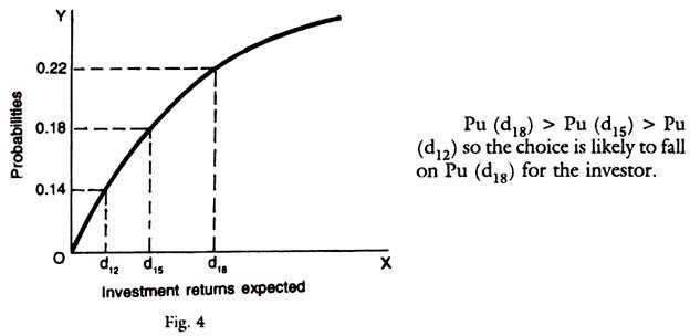
Based on some assured values of expected return and their probabilities, one can draw a graph depicting their relationship. The investor will choose that alternative with the highest value of Pu (di) – a utility maximising function.
The following chart explains this:
The basic assumptions of the utility analysis are:
(1) Utility is measurable although it is subjective.
(2) Investor always prefers more terminal wealth to less terminal wealth — principle of non-satiation is accepted.
(3) Investors are normally risk averse.
(4) Investors behave rationally so as to maximise expected utility consistent with their risk tolerance.
(5) Normally investors put some money in the riskless assets whose expected returns are less but distribute the rest of the money in a stochastic manner in assets which yield positive expected returns, so that the investors make choices involving risk that maximise their expected utility.
There will be positive but diminishing marginal utility of wealth and decreasing absolute risk aversion. Generally such functions are positive monotonic functions which are concave toward wealth axis. As marginal utilities are decreasing with increasing investments, the investor will invest in each of the assets upto the point that marginal utilities in each of the lines of investment are equal and positive.
It is seen from the above that the Investor’s expected utility could be expressed as a function of risk, measured by standard deviation of returns and expected returns. Given the value of σ2 (risk) and r (return) for a number of alternative portfolios, the investor can depict his choices giving equal satisfaction on what is called an Indifference Curve.
ii. Indifference Curve Technique:
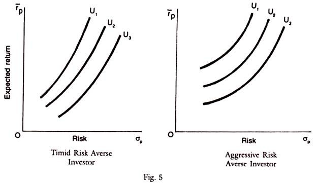
Investor’s expected utility can be expressed as a function of risk, measured by the Standard deviation of returns. The indifference curve is a locus of points on which the investor is indifferent between utility as return expected and its expected risk. This curve reflects the relationship of rp with σp , rp is drawn on the y-axis and σp on the x-axis, as shown below. Indifference curves can be derived from the investor’s utility function and used to represent investor’s preferences for risk and expected return.
An investor can have a set of Indifference Curves, where each curve corresponds to a given level of expected utility. Expected utility will increase as one moves from one curve to another higher curve, in the sense that it lies in the north westerly direction for risk averse investors. As the normal investors are risk averse, their indifference curves are convex and positively sloped.
But there are many risk takers who are inclined to take higher levels of risk and these are called risk seekers. For them, the indifference curve will be concave and negatively sloped, the investor can have any number of possible portfolios, each with its own expected return and risk. He prefers that one which gives higher return for the same risk or lower risk for a given return.
To sum up, an indifference curve is the locus of all possible portfolios that provide the investor with the same level of expected utility. Expected utility will increase as one moves from lower indifference curve to a higher indifference curve. But on the same indifference curve any point on the curve gives the same utility. Such curves are positively sloped and convex for risk averters, concave for risk seekers and horizontal for risk neutral investors.
iii. Efficient Frontier:
Each security has an expected return (r) and risk (σi) value connecting these securities with lines representing all possible combinations constituting the portfolios generates the opportunity set for the Investor. Within the opportunity set, are all individual securities as well as portfolios. The outer boundary of an opportunity set is called the efficient Frontier line and within the boundary are all possible sets.
G.J. Alexander and J.C. Francis define an efficient portfolio as:
“one which has greater expected return than any other portfolio in its risk class or one which has less risks than any other portfolio with the same level of expected return.”
The curvature of efficient frontier is concave which follows from the covariance effect in that if one moves to higher values of portfolio (Er) that will reduce the number of securities that can be held in combination so as to lower a (risk). If the curvature is not concave, one can move from a lower return to a higher return for a given level of risk. At the outer points of the concave curve, one gets the most efficient points. This curve has to be concave only under the given assumptions, just as the Indifference Curve has to be convex to the origin for a rational risk averting investor.
The assumptions may be summarised as follows:
1. A rational investor is risk averse.
2. He tries to maximise his expected utility.
3. He chooses the optimal portfolio on the basis of lowest risk (o) or standard deviation of returns (r).
4. Markets are perfect and information is free with no transactions costs and no taxes.
5. The time horizon is known and fixed.
Importance of Covariance Term:
For a portfolio of securities, it is not only the expected returns and variances that matter but the covariances as between these securities in the portfolio. The variances of a weighted sum are not always simply the sum of the weighted variances, since the covariance term, shown below may increase, or decrease the total sum.
Thus, the equation is as follows:
The covariance term is crucial in Modern Portfolio Theory and particularly in diversification of Markowitz type. If covariance is zero, the weighted sum of variances is not changed. If it is more than one and positive, risk is increased. If it is less than one or negative, risk is decreased. The covariance and its importance is brought out in the Markowitz Theorem of Diversification. In the words of Markowitz, “Not only does the portfolio analysis imply diversification, it implies the right kind of diversification for the right reason… in trying to make variance of returns small, it is not enough to invest in many securities. It is necessary to avoid investing in securities with high covariances among themselves.”
The indifference curves are convex and efficient frontier lines are concave and that the efficient Frontier Theorem postulates that the optimal portfolio for a risk averse investor must be located on the efficient frontier.
This is graphically shown as follows:
EMF is the Frontier line and M is the optimal portfolio where I2. Curve runs tangential to efficient frontier line.
The P and M maximises the utility, for a given level of risk. Any point below M is feasible but gives less return for the same risk (σp). Any point above M is not feasible due to wealth constraint. Investor prefers to be on a higher Indifference curve I1 than an I2 but it is not feasible, as it does not touch any of the possible efficient sets of portfolios. The point of tangency of the utility curve (or I2) with the efficient frontier line EF determines the choice of the portfolio which is optimal for his given choices and preferences.
In the above graph, it is assumed that there is no lending and borrowing and that the investor invests all his funds in risky securities, as this model does not take into account the possibility of risk free investment and borrowing and lending at risk free rates.
The importance of covariance in the language of common man is the relative interdependence in terms of risk of the securities within the given portfolio. Thus, one can diversify into three companies in steel which will have more risk than three companies in three industries, say steel (Tisco), cement (Indian Cement) and pharmaceuticals (Dr. Reddy Labs). The reason is that in the former case all the scrips have similar risks and the sum of the risks is say y (x1 + x2 + x3) and the covariance between x1 and x2, x2 and x3 and x1 and x3 is positive and high, which makes the total sum of all risks higher than (x1 + x2 + x3).
In the latter case, the risk in cement industry is different from that of steel and pharmaceuticals. Even if steel and cement are complementary, that of pharmaceuticals will be different and covariance between cement (y1) steel (y2) and pharmaceuticals (y3) may be low or negative which will reduce the sum of the total risks to less than (y1 + y2 + y3). Thus, covariance as between the scrips included in a portfolio makes a lot of difference to the diversification technique.
As per Markowitz diversification, the term covariance makes all the difference to the sum total risk of all risks in a portfolio because the covariance may increase or decrease the sum of the risks of scrips in a portfolio. Tobin introduced the possibility of existence of a security with no risk.
For a two security portfolio, the standard deviation can be calculated by using the following equation:
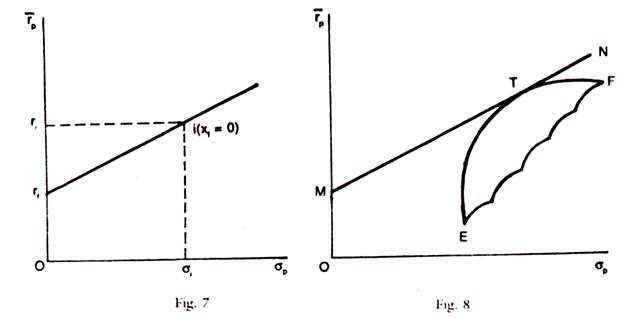
The graph in the case of only one risky asset x( is shown in Graph 7 and risk free borrowing and lending, is shown in graph 8.
Expected returns are shown in Y-axis and risk is represented on X-axis.
M N is the line showing free borrowing and lending and E F is the efficient frontier.
The positions with Risk free borrowing and lending with a single risky asset i is shown in the graph below.
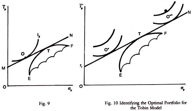
Risk free borrowing and lending with the Markowitz Model (Tobin Model). The following graph shows the identification of optimal portfolio for the Tobin Model, at the point T (Graph 9).
Any efficient frontier line is combined with the risk free asset or risk free borrowing and lending, in Graph 10. The graphs are self explanatory.
At O* this portfolio involves investing 50% of the investor’s funds in risk free asset and 50% in portfolio T. Next at point O**, this portfolio involves borrowing an amount equal to 50% of investor’s own funds and investing the borrowed funds and investor’s own funds at point T. In this case and in general efficient lending and efficient portfolios above T involve risk free borrowing.
