Cournot Model and Stackelberg Model (With Diagram)

The Cournot Model and the Cournot Solution:

The first systematic oligopoly model was published by the French economist Antoine Augustin Cournot (1801-77) in 1838. Although Cournot’s model was based on some unrealistic assump­tions, his method of analysis has been useful for subsequent theoretical development in the areas of duopoly and oligopoly.

The Assumptions of the Cournot Model:

The Cournot model is based on the following assumptions:

(i) There are only two non-collusive firms, i.e., there exists the simplest example of oligopoly, viz., duopoly.

(ii) The two sellers (duopolists), say A and B, are producing homogeneous goods.

The model’s other assumptions (from which most of the models discussed hereafter will draw) are:

(iii) The product is perishable, i.e., they cannot be stored and must all be sold within the duration of the period.

(iv) There are many knowledgeable buyers of the product.

(v) Each duopolist knows the market demand curve for the product.

(vi) The two firms have identical cost curves and, for the sake of making the matter simple, we shall assume that the cost of producing each output is zero for both the firms.

(vii) Each firm makes an output plan at the beginning of each period, and it cannot revise the plan within the duration of the period.

(viii) Neither of the firms sets a price for its product, and each accepts the price at which the total planned output can be sold.

(ix) Each duopolist wants to earn the maximum profit in each period.

(x) While the duopolists are aware of mutual interdependence of their output plans, each is quite ignorant of the direction and magnitude of the revision in his rival’s plan that would be induced by any given change in his own. We shall suppose, therefore, that each duopolist assumes that, irrespective of his output plan in any period, his rival will maintain his output at the same level as in the previous period.

The Iso-Profit Curves:

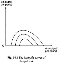
On the basis of assumptions, we shall obtain the iso-profit curves of each duopolist. As the name suggests, an iso-profit curve of a duopolist, A, gives us the combi­nations of outputs of the duopolists A and B, which would yield the same amount of profit for duopolist A.

The iso-profit curves of A would look like those given in Fig. 14.1, where the output of A is measured along the horizontal axis and that of B along the vertical axis.

The points on any one of these curves are the combinations (q_A, q_B) of the per-period outputs of the duopolists that give A the same amount of profit per period. In other words, each iso-profit curve of a duopolist represents a particular amount of profit, and we shall see that a lower iso-profit curve of A (i.e., one nearer the horizontal axis) would give him a higher amount of profit.

But let us first explain the shape of the iso-profit curves that are given in Fig. 4.1. In order to do that, we have to understand the relation between the outputs and profits of the duopolists, A and B, subject to the assumptions given above.

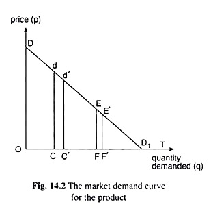
In Fig. 14.2, the market demand curve for the product has been given to be DD_b and OC is any particular quantity of output of duopolist B. Since each duopolist assumes the output of his rival to remain constant at where it is, the relation between A’s output (q_A) and the price of the product (p) would be given now by the segment dD₁ of the market demand curve DD₁.

For example, if A produces and sells CF quantity of output, then the total quantity of output sold would be OF, and we can know from the demand curve, DD₁, that the price of the product at this quantity would be EF.

Therefore, under the circumstances, duopolist A’s demand curve would be dD_c and the quantity-axis and the price-axis of this demand curve would be, respectively, CT and Cd. Now, if E be the midpoint of segment dD₁, then B’s output (q_B) remaining the same at OC = constant, if q_A increases from zero onwards (and p diminishes), A’s total revenue (R_A) and total profit (π_A) would also increase till q_A becomes equal to CF.

This is because the numerical coefficient of price-elasticity of demand (e_A) is greater than one (e_A > 1) over the segment dE of A’s demand curve, and the total costs of the duopolists (C_A and C_B) at each output are zero [assumption (vi)].

If q_A increases beyond the quantity CF (and p diminishes), then A’s total revenue (R_A) and total profit (n_A) would be decreasing, since, over the segment ED] of his demand curve, e_A is less than one (e_A < 1). At the point E on A’s demand curve dD₁ we have = 1 and marginal revenue of A (MR_A) = 0, and so, at E, R_A and π_A are maximum.

Similarly, if in Fig. 14.2, the specific quantity of output of duopolist B be OC’ (OC’ > OC), then A’s demand curve would be the d’D₁ segment of the market demand curve, DD₁. Along this demand curve, as q_A increases (and p diminishes) over the range C’F’, R_A, and also π_A, increases, since over the segment d’E’ of his present demand curve, d’D₁, he has e_A > 1.

At the point E’, which is the midpoint of the segment d’D₁, e_A = 1 and, therefore, R_A, and also π_A, is maximum. Now, we have to note here:

Now, since it is evident that C’D₁ < CD₁, we obtain C’F’ < CF. That is, as the given quantity of B’s output increases (OC’ > OC), the profit-maximising output of A diminishes (C’F’ < CF).

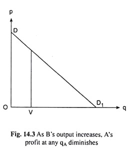
We shall now see what would be the effect of an increase in B’s output (q_B) upon A’s profit when A’s output (q_A) remains constant at some particular quantity. In Fig. 14.3, DD, is the market demand curve for the product and A’s output (q_A) is OV = constant.

In this case, as B increases his output from zero to VD₁, the price of the product (p) would be diminishing and also R_A = π_A from the sale of the output of q_A = OV = constant, would be diminishing.

Therefore, in the above discussion, we have obtained:

(i) If q_B remains unchanged at any particular quantity (e.g., OC in Fig. 14.4), then as q_A increases, π_A would rise at first; then at some output (like CF), π_A would be maximum. If A’s output increases further, π_A would be falling.

(ii) The larger the fixed quantity of q_B the smaller would be the profit-maximising quantity of q_A. For example, for OC’ > OC, we have obtained C’F’ < CF.

(iii) If q_A remains constant at a particular quantity like OV in Fig. 14.3, then π_A would be falling as q_B increases.

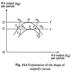
On the basis of the above points, we shall now be able to arrive at the shape of the iso-profit curves of the duopolist A. Two of these curves are shown in Fig. 14.4. In this figure, duopolist A’s output per period has been measured along the horizontal axis and B’s output per period has been measured along the vertical axis.

In other words, the points in the output space of Fig. 14.4 represent different combinations of the outputs of A and B. Therefore, each point in this space implicitly represents a combination of R_A and R_B and, so, of π_A and π_B.

Let us now represent what we have obtained in Fig. 14.2 in a separate diagram, viz., Fig. 14.4. In Fig. 14.4, at q_B = OC = constant, A would have to produce an output of CF in order to obtain the maximum profit, i.e., the output combination or the point F (CF, OC) lying on the horizontal line, Cx, would give A the maximum profit at q_B = OC.

As we already know, B remaining constant at OC, as q_A increases from zero to CF, π_A increases, and then, as q_A increases beyond CF, π_A decreases. Therefore, at the points on the line Cx to the left or right of F, e.g., at points H₁ or H₂, A’s profit would be less than that at the point F.

Now at the point H₁, i.e., at the output CH, (CH, < CF), the firm A may obtain the same profit as at F, if B’s output diminishes sufficiently, say, by H₁T₁, from the level of OC, for, if q_B diminishes, the price of the product would increase.

Therefore, π_A may be the same at the points F and T₁, i.e., an iso-profit curve of A may pass through the points T₁ and F. Similarly, if q_B diminishes sufficiently, say, by H₂T₂, from the level of OC, π_A may be the same as at point F. Therefore, the iso-profit curve through T₁ and F may also pass through the point T₂.

Therefore, how we may obtain the output combinations of the duopolists that give A the same profit as at the point F, and we have obtained that the curve T₁FT₂ is one of the iso-profit curves of duopolist A. This curve would be concave to the horizontal axis and the highest point of the curve would be F.

It is obvious from the construction of the iso-profit curve T₁F T₂ that the horizontal line Cx touches this curve at the point F. Also, F is the maximum (highest) point of the iso-profit curve T₁FT₂, since a horizontal straight line (Cx) may touch a concave downward curve (like T₁FT₂) only at the latter’s maximum point.

In order to complete our explanation of the geometry of the iso-profit curves, we have to draw another curve like T₁F T₂. As we have already obtained in Fig. 14.2 and now represented in Fig. 14.4, at q_B = OC’ = constant (OC’> OC), the profit-maximising output of A is C’F’ (C’F’ < CF).

That is now at B’s output = OC’ = constant, A’s profit-maximising output would be obtained at the point F’ on the horizontal straight line C’x’. Proceeding in the same way as in the previous case, we will find that profit levels at the points T₃ and T₄ would be the same as that at the point F’.

Therefore, the curve T₃F’T₄ becomes another iso-profit curve of duopolist A. As in the previous case, the line C’x’ would touch this curve at the latter’s maximum point, F’.

In Fig. 14.4, we have now obtained two iso-profit curves of duopolist A. The general features of these curves (of any duopolist) may now be systematically listed:

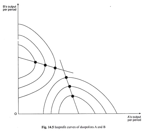
(a) The iso-profit curves of a duopolist would be concave to the axis along which his output is measured. In Fig. 14.5, we have measured output of duopolist A along the horizontal axis. So A’s iso-profit curves would be concave to this axis. Similarly, if we measure output of duopolist B along the vertical axis, the iso-profit curves of B would be concave to the vertical axis.

(b) In Fig. 14.4, we have obtained: C’F’ < CF. That is, the maximum point F’ of the higher iso-profit curve of A would be nearer the vertical axis than the maximum point F of his lowest iso-profit curve. Similarly, the farther an iso-profit curve of B would be from the vertical axis, the nearer its maximum point would be to the horizontal axis.

(c) The higher iso-profit curve of a duopolist represents a lower profit level. This is obtained from point (iii) above which gives us that, q_A remaining constant at a particular quantity, A’s profit (π_A) would be falling as q_B rises. Similarly, a higher iso-profit curve of duopolist B would represent a lower level of profit. Therefore, a profit-maximising duopolist would strive to reach the lowest possible iso-profit curve.

Some of the iso-profit curves of duopolists A and B that assume the above features, have been shown in Fig. 14.5.

The Cournot Reaction Functions Derived from the Iso-Profit Curves:

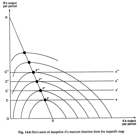
In Fig. 14.6, we have drawn some iso-profit curves of duopolist A. This figure may also be called the iso-profit map of duopolist A. From this iso-profit map, we would obtain a function that would express A’s output per period (q_A) as a function of B’s output (q_B). This function is called the (Cournot) reaction function of duopolist A.

We may now see how we can obtain the reaction function of duopolist A from his iso-profit map given in Fig. 14.6. As we already know, if q_B is given to be, say, OC = constant, then the duopolist A’s profit-maximising output would be given by the point of tangency, F, between the horizontal straight line Cx and one of his iso-profit curves, here If. For, at the point F, the firm is on the lowest possible iso-profit curve, i.e., on the highest possible level of profit subject to B’s output = OC = constant.

Now, if B’s output increases from OC to, say, OC’, A’s profit-maximising output would be given by the point F’ which is the point of tangency between the horizontal straight line C’x’ and one of the iso-profit curves, viz, I^A₂ .

We have obtained, therefore, that if q_B is OC then A’s (profit-maximising) output, q_A, would be CF and if q_B is OC’, then q_A would be C’F’. Similarly, we would obtain that if q_B is OC” and OC'”, then q_A would be, C”F” and c'”F'” respectively, and so on.

We, therefore, obtain here q_A as a function of q_B. The line that would give us this reaction function of duopolist A would be one that joins the points like F, F’,F”,F”‘, etc. In Fig. 14.6, this reaction function of A has been obtained to be the line RS.

It would be a straight line if, the market demand curve for the product is a straight line, and it would be negatively sloped, because, as B’s output increases, profit-maximising output of A diminishes.

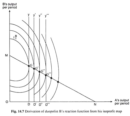
We have seen above how we may obtain the reaction function of duopolist A. We may obtain the reaction function of duopolist B also following the same procedure. This function would give us the profit-maximising output of B as a function of A’s output. We have done this in Fig. 14.7 where we have been given the iso-profit map of duopolist B.

In this figure, at q_A = OD = constant, the profit maximising output of B (q_B) would be obtained at the point of tangency, G, between the vertical straight line Dy and one of B’s iso-profit curves, viz., If . For, at the point G, B is on the lowest possible iso-profit curve subject to q_A = OD.

Similarly, as q_A increases to OD’, OD”, OD'”, etc., q_B would be given respectively by the points G’, G”, G”‘, etc. If we join these points by a line, we would obtain the reaction function of B, which would give B’s output as a function of that of A. B’s reaction function like that of A’s would also be a negatively sloped straight line if the market demand curve for the product is linear.

Mathematical Derivation of the Cournot Reaction Functions:

On the basis of the assumptions made in the Cournot model, we may now derive mathemati­cally the Cournot reaction functions.

Let us suppose that the market demand curve for the product is

where p = price of the product

q = quantity of market demand for the product

q_A = quantity sold by duopolist A

q_B = quantity sold by duopolist B

a = vertical intercept of the market demand curve (14.9) = positive constant

-b = slope of the market demand curve (14.9) = negative constant

For the sake of simplicity, we have assumed here that the market demand curve (14.9) is a (negatively sloped) straight line.

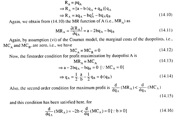
By definition, the TR (or simply R) function of the duopolist A (i.e., R_A) is

Equation (14.14) gives us that the profit-maximising (or equilibrium) output of duopolist A(q_A) is a function of the output of duopolist B(q₀), i.e., from this function, we are able to know the output of A at any particular quantity of output of B. In other words, (14.14) is the reaction function of duopolist A.

As is evident from the form of equation (14.14), the reaction function of A has been obtained as a (negatively sloped) straight line (like RS in Fig. 14.6).

This is because we have assumed here that the market demand curve for the product is a (negatively sloped) straight line.

As we may see from equations (14.9) to (14.14) that if the market demand curve (14.9) is a straight line, then the R_A function (14.10) is a second degree curve and the MR_A function (14.11), being the derivative of R_A w.r.t. q_A, would be a straight line, and this straight line MR_A function leads to a straight line reaction function (14.14) when we put MR_A = MC_A = 0.

Now, the reaction function of duopolist B would be obtained in the same way, and this reaction function would be

Like the reaction function (14.14) of duopolist A, the reaction function (14.17) of duopolist B would also be a straight line like MN in Fig. 14.7.

Equilibrium in the Cournot Model—Competitive, Monopoly and Duopoly Solutions:

We have seen above that the reaction functions of the duopolists have been derived from the profit-maximising conditions, and by assumption, both the duopolists pursue the profit- maximising goal. Therefore, both of them would intend to remain on their respective reaction functions.

Under the circumstances, equilibrium in the Cournot model can occur only at the point of intersection of the two reaction functions. In other words, the equilibrium combination of the outputs of the two sellers would be obtained if we solve the two reaction functions for q_A and q_B. But before doing this, let us note the following.

As we know, the condition for a competitive equilibrium is p = MC. In the Cournot model, at each value of q_A and q_B, we have assumed MC_A = MC_B = 0 [assumption (vi)]. That is why, at any output of the two firms taken together, i.e., at any q = q_A + q_B, we would have MC = 0. Therefore, here the condition for competitive equilibrium would be p = MC = 0.

Therefore, if we put p = 0 in (14.9), we would obtain the competitive solution (output) in the Cournot model:

q_c = a/b                                            (14.18)

Next, let us note the significance of the intercepts of the Cournot reaction functions, which, as we know, are negatively sloped, i.e., as the output of one seller increases, the profit-maximising output of the other seller decreases.

Let us suppose now that the reaction functions of A and B are RS and MN in Figs. 14.6 and 14.7. We obtain from the reaction function RS that, as q_B rises to OR, q_A reduces to zero. If we put q_A = 0 in the reaction function of (14.14) of A, we obtain

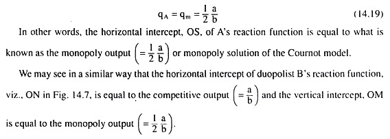
That is, as q_B rises to OR = a/b, q_A falls to zero. In other words, the vertical intercept OR of A’s reaction function is equal to the competitive output. Again, we obtain from A’s reaction function that, as the output of B reduces to zero, and A becomes a monopolist, i.e., as the duopoly becomes a monopoly, output of A rises to OS which is called the monopoly output.

Therefore, if we put q_B = 0 in A’s reaction function, we obtain the monopoly solution (q_m) of the Cournot model as

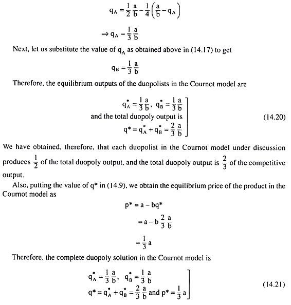
Let us now solve the Cournot reaction equations (14.14) and (14.17) for the equilibrium values of q_A and q_B. Substituting from (14.17) into (14.14), we obtain

Geometrical Presentation of the Equilibrium Solution in the Cournot Model:

Cournot’s solution is based on his assumptions. The last assumption [i.e., assumption (x)] may be called the key assumption of the model. This assumption is very naive for it implies that the duopolists do not learn from experience—they stick to the belief that the rival would maintain his output at the level of the previous period although they repeatedly prove wrong.

However, as we shall see, the last assumption, although naive, gives the Cournot model a determinate solution.

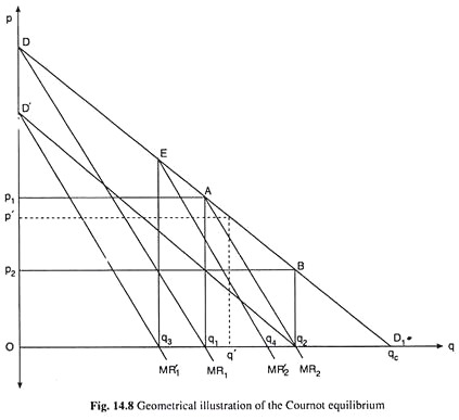
Cournot’s explanation is based on the example of mineral water from two adjacent springs. The mineral water is produced at zero long-run marginal cost. His analysis is illustrated by means of Fig. 14.8, where the market demand curve for the product is given to be DD₁.

The MR curve associated with this demand curve is MR₁. Since MC = 0, the competitive output here is the q at which p = MC = 0. Therefore, the competitive output is obtained to be Oq_c in Fig. 14.8.

The monopoly output, on the other hand, is one at which the condition MR = MC = 0 is satisfied. Therefore, the monopoly output here is Oq₁ and the monopoly price is Op₁, and the monopoly profit is the total revenue area Op₁Aq₁, since total cost by assumption is zero. The monopoly solution would be the solution if the two duopolists colluded and formed a multi-plant monopoly.

However, Cournot’s solution to the duopoly problem proceeds as:

Let us suppose that initially, i.e., in period 0, A is the only seller in the market. He, therefore, behaves like a monopolist and produces the monopoly (MR = MC = 0) output, Oq₁ = 1/2 Oq_c, and sells at a price, Op₁, and makes a profit equal to area Op₁Aq₁. In period 0, therefore, we have A’s output = Oq₁ and B’s output = 0.

Let us now suppose that, in period 1, B enters the market. By assumption (x), he would expect A to produce and sell his output of the previous period, i.e., Oq₁, and A would actually produce Oq₁ assuming that there would be no rival as in the previous period. Now if B produces in period 1, he cannot sell anything at or above the price, Op₁. At a price less than Op₁, B can sell the quantity demanded in excess of Oq₁.

For example, at a price of Op’, B can expect to sell q₁q’. The demand curve for duopolist B would be the segment AD₁ of the market demand curve DD₁ with origin at q₁. His marginal revenue curve would be MR₂ with origin again at q₁.

Since he would produce and sell at the MR = MC (= 0) point, his output would be q₁. Total duopoly output now would be Oq₂. Since total output has increased, price would fall from Op₁ to Op₂. In period 1, therefore, A proves wrong and B correct. In this period, we would have A’s output = Oq₁ and B’s output = q_tq₂.

As B has now entered the market, and because of his entry, supply of the product has increased and price fallen, A would revise his production plan in the next period, i.e., in period 2. Again, by assumption (x), A would assume that B would continue to produce the output of q₁q₂ = q₂q_c, which B would actually do assuming A’s output to be Oq₁.

Therefore, in period 2, A would have to relocate his demand curve by horizontally shifting DD₁ leftward to D’q₂ by the amount q₂q_c (= q₁q₂) i.e., he would now re-determine his demand function by subtracting the amount q₂q_c from each quantity of his original demand.

The new MR curve of A now would be MR₁ and his new output quantity would be determined at the MR = MC (= 0) point and it would be Oq₃ = 1/3 Oq₂. As there is now B in the market, A has reduced his output from Oq₁ to Oq₃. In period 2, therefore, A has proved correct and B has proved wrong. In this period, we would have A’s output = Oq₃ = 1/2 Oq₂ and B’s output = q₁q₂.

Therefore, in period 3, B would reevaluate the situation. His new demand curve would be the segment ED₁ of the market demand curve, DD₁ with origin at q₃ and his MR curve now would be MR₂ with the same origin.

Therefore, now he would produce the output q₃q₄, which would be determined at the MR = MC (= 0) point. In this period, then A proves wrong and B proves correct. Now, we would have A’s output = Oq₃ = 1/2 Oq₂ and B’s output = q₃q₄.

This process would go on in the Cournot model, A’s output decreasing and B’s output increasing until both A and B produce the same output of 1/3 q_c. The Cournot model will be in equilibrium when each duopolist produces an output of 1/3 q_c and the total output would be 2/3 q_c where q_c (or Oq_c) is the competitive output.

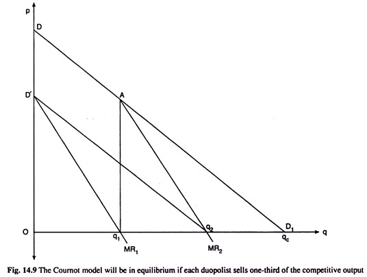
We may now easily verify that if each duopolist produces an output of 1/3 Oq_c, then the Cournot model will be in equilibrium. In Fig. 14.9, the market demand curve is DD₁ and the competitive output is Oq_c, as they were in Fig. 14.9.

Now if the duopolist A produces the output Oq₁ = 1/3 Oq_c, then the duopolist B’s demand curve would be the segment AD₁ of the market demand curve DD₁ and his MR curve would be MR₂, both with origin at q₁. Therefore, B would produce an output of qjq₂ at the point MR = MC (= 0). But we have q₁q₂ = 1/2 q₁q_c = 1/2 . 2/3 Oq_c = 1/3 Oq_c.

That is, if A produces 1/3 Oq_c, the profit-maximising output of B would also be 1/3 Oq_c. Let us now see, what would be the output of A if B’s output is given to be q₁q₂ = q₂q_c = 1/3 Oq_c.

If B produces q₂q_c, then, A would horizontally shift the demand curve DD₁ leftward by the amount q₂q_c, and it would become D’q₂ for A and the corresponding MR curve would be MR₁, both with origin at O. A would now produce at the point where he has MR = MC (= 0) and so his output would be 1/2Oq₂ = Oq₁ = 1/3Oq_c.

Therefore, that if A’s output is 1/3 Oq_c, B would produce an output equal to 1/3 Oq_c; and if B’s output is 1/3 Oq_c, then A would produce an output equal to 1/3 Oq_c. That is, along the approach road to equilibrium, when one of the duopolists happens to produce 1/3 of the competitive output, then the other firm would also produce the same output, and the Cournot model will be in equilibrium.

Together, the duopolists would produce 2/3 of the competitive output (Oq_c).

Equilibrium of the Cournot Duopoly Market—an Alternative Geometrical Illustration:

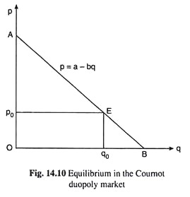
We may now illustrate the equilibrium in the Cournot duopoly market with the help of Fig. 14.10. In this figure, the straight line AB is the market demand curve (14.9) for the product.

Here OA = a and OB = a/b. Let us now suppose p* = 1/3a = OA = Op0 and q* = 2/3 a/b = 2/3 OB = Oq0 [eqn (14.21)]. Therefore, Fig. 14.10, the equilibrium point in the duopoly market is E (p = Op₀, q = Oq₀).

In the Cournot model, by assumption (x), each duopolist fixes his output in any particular period, by assuming that his rival would keep his output unchanged at the quantity he produced in the previous period.

In spite of this assumption proving wrong repeatedly in reality, if the duopolists cling to this assumption, then eventually in some period, their assumption would prove correct, and both of them would reach the equilibrium point. We may illustrate the process with the help of Fig. 14.11.

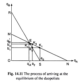
In Fig. 14.11, the outputs of A and B (q_A and q_B) are measured, respectively, along the horizontal and the vertical axis. Here, the straight line RS is the reaction curve of duopolist A. From this curve, we can know what would be the equilibrium output of A at any given output of B. Similarly, the straight line MN is the reaction curve of duopolist B. This curve would give us the equilibrium output of B at any given output of A.

Let us note that RS and MN are the reaction curves corresponding to the reaction functions (14.14) and (14.17), respectively. By definition, both OR and ON represent the competitive output in the Cournot model. That is why OR would be equal to ON in Fig. 14.11. Again, both OS and OM represent the monopoly solution of the model [14.2.2(d)], and so here OM would be equal to OS.

We may now illustrate how and along what path the duopoly firms would approach their equilibrium. Initially (in period 0), there is no B, and duopolist A would behave like a monopolist. His reaction function (RF) gives us that at q_B = 0, q_A = OS (or Oa₀)—this is the monopoly solution.

Let us now suppose that in period 1, duopolist B enters the market and begins to produce the commodity. So the market now becomes duopolistic. In period 1, firm A would produce q₁ = OS (or Oa₀) as in the previous period, assuming that B’s output, q_B, would be zero and B would produce the output, Ob₁, assuming that A would produce the previous period’s output, OS.

The output combination that would be produced in period 1, would therefore, be K₁ (Oa₀, Ob₁). In this period, A would prove wrong and B would prove correct in their assumptions about each other’s production plan.

In period 2, duopolist A would revise his production plan for he proved wrong in period 1. In this period, A would produce Oa₂ assuming that B would produce his period 1 output, i.e., Ob₁, and B would actually produce Ob₁ (wrongly) assuming that A would produce his period 1 output, i.e., Oa₀.

The output combination in period 2, therefore, would be K₂(Oa₂, Ob₁). In period 2, A would prove correct in his assumption about B’s output, but B would prove wrong in his assumption about A’s output.

Similarly, in period 3, B would revise his output plan for he proved wrong in period 2 in his assumption about A’s output. In period 3, B would produce ob₃, assuming that A would produce his previous period’s output, Oa₂, and A would actually produce this output (Oa₂), assuming (wrongly) that B would produce his period 2 output, viz., Ob₁, The output combination in period 3, therefore, would be K₃(Oa₂, Ob₃).

In this period, A would prove wrong and B would prove correct.

The adjustment process that we have underlined above would go on so long as one of the duopolists would prove wrong although the other one proves correct—the output combination would move from the point K₁ on MN to K₂ on RS to K₃ on MN, and so on.

As we see in Fig. 14.11, ever since B entered the market, A’s output has decreased in the adjustment process and B’s output has increased, and so, the output combination would alternately move first from B’s RF to the west on A’s RF (as from K₁ to K₂) and then from A’s RF to the north on B’s RF (as from K₂ to K₃) and then again to west, and so on, till the output combination becomes E (q *_A, q*_B) at the point of intersection of the two reaction curves, where the output quantity of each duopolist would be obtained to be q*₁ = q*₂ = 1/3 a/b [eq. (14.20)].

Since E lies on the RFs of both the duopolists, once one of them produces q*_A = q*_B = 1/3 a/b, the other would also produce q*_A = q*_B, i.e., if A produces q*_A, B would produce q*_B and if B produces q*_B, A would produce q*_A, and thus it would go on.

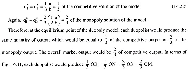
Therefore, E is the equilibrium point of the Cournot model of duopoly, where each duopolist would produce:

Critical Comments on the Cournot Model:

Let us note that Cournot’s model can be generalized into an oligopoly model with more than two firms. The model may also be extended to positive marginal cost.

Let n be the number of oligopolists (n > 2), q_c the competitive output, p_c the competitive price, and p_m the monopoly price. Then the total output in Cournot equilibrium under oligopoly would be nq_c/n +1. Each firm’s output would be q_c/(n+1), and the price in the oligopoly market would be 2p_m/n+1 + np_c/n+1.

In the duopoly model, we had n = 2 and p_c = 0. Also, as the number of firm’s (n) tends to infinity and the model tends to become a competitive market model, n/n+1 would tend to 1. Hence, the total output, as expected, would tend to become q_c, the competitive output, and the price would tend to become p_c.

Second, in the Cournot model, each duopolist believes that the rival will not change his output. This was criticised by a French mathematician Joseph Bertrand. Bertrand argues that a more realistic assumption would have been that each duopolist believes that his rival will not change his price.

Along with this assumption, Bertrand brings in only one more assumption which states that each duopolist has sufficient capacity to satisfy the entire market. In this model, A will first start with the monopolistic price; B then enters the market, reducing the price somewhat, and captures the whole market.

A then lowers the price below B’s level and captures the market, and the process will continue. Finally, the price war ends when price comes down to the level p = MC = 0, and the total output produced becomes equal to the competitive output.

Chamberlin also changes Cournot’s assumption that each duopolist naively believes that his rival’s output would remain unchanged. Instead, he simply assumes that the duopolists are aware of their interdependence.

He argues like this:

A starts with output Oq₁ and price Op₁ in Fig. 14.8, and B produces q₁q₂, as was the case with Cournot. A, however, then realizes that B will change his behaviour if A changes his output, and that the maximum joint profit occurs at the output level Oq₁.

A, therefore, cuts his output level to 1/2 Oq₁ leaving B to produce 1/2 Oq₁ = q₁q₂. A stable solution is thus obtained, which is the monopoly solution. Here, there is no explicit collusion. There is only some understanding of mutual benefit. In the Cournot model, however, there is no scope for price competition since here the duopolists are price-takers.

Third, in the Cournot model, a duopolist is not able to make any guess about the rival’s reactions to a change in his own output. He, therefore, cannot make any conjecture about his rival’s behaviour, i.e., he does not behave conjecturally.

He rather behaves autonomously for he assumes that his rival’s output is given autonomously. Of course, this autonomous behaviour takes both of them to the intersection point of their reaction functions where they would be in equilibrium, i.e., ultimately they would prove right, although for wrong reasons.

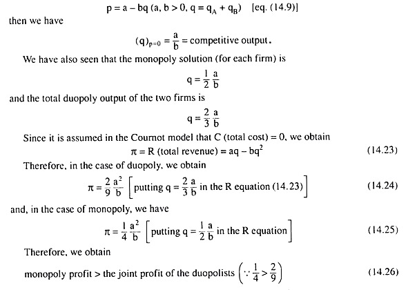
Lastly, we should note that although the duopolists in the Cournot model are able to maximise their individual profits subject to the given assumptions, their joint profit and, therefore, their individual profits (obtained after the joint profit is appropriately distributed), might have been larger if they acted collusively and formed a multi-plant monopoly. This we can prove very simply in the following way.

If the market demand curve for the product is

The Cournot Solution—Non-Zero Costs:

The basic behaviour assumption of the Cournot model is that each duopolist maximises his profit on the assumption that the quantity produced by his rival does not depend on his own quantity decision.

That is, duopolist A maximises π_A w.r.t. q_A, treating q_B as a constant, and duopolist B maximises k_b w.r.t. q_B, treating q_A as a constant. We may now obtain the Cournot solution for the market model given by equations (14.1)—(14.4).

Setting the appropriate partial derivatives of the n equations in (14.3) equal to zero, we obtain

 

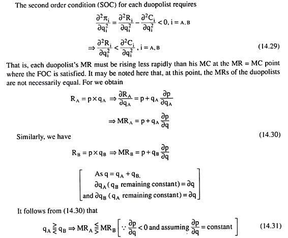
That is, the duopolist with the greater output will have the smaller MR, and the MRs of the duopolists will be equal if they produce and sell the same quantity of output. The duopolistic market will be in equilibrium if the values of q_A and q_B are such that each duopolist maximises his profit given the output of the other, and neither desires to alter his output.

The equilibrium solution can be obtained if we solve the FOCs (14.28) for q_A and q_B, provided the SOCs (14.29) are satisfied. However, the Cournot solution may be better represented and better explained if we proceed through the reaction functions.

Reaction functions, by definition, express the output of each duopolist as a function of his rival’s output. As such, the reaction function of duopolist A would be obtained if we solve the first equation of (14.28) for q_A in terms of q_B and the reaction function of duopolist B would be obtained if we solve the second equation of (14.28) for q_B in terms of q_A. These two functions may be written as

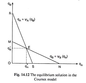
Duopolist A’s reaction function gives the value of q_A for any specified value of q_B, which maximises π_A. Similarly, duopolist B’s reaction function gives the value of q_B for any specified value of q_A, which maximises π_B. The equilibrium solution of the Cournot model, as we already know, is obtained at the point of intersection of the two reaction functions. This equilibrium solution is a (q_A, q_B) combination.

Let us denote this combination by E (q_A, q_B) in Fig. 14.12. Since this combination lies on the reaction function of duopolist A, A sells q*_A, given q_B = q*_B, and maximises his profit (π_A). Again, since the combination E lies on the reaction function of duopolist B, B sells q*_B, given q_A =q*_A, and maximises his profit (π_B). Therefore, when they arrive at point E, neither of them would be willing to alter his output.

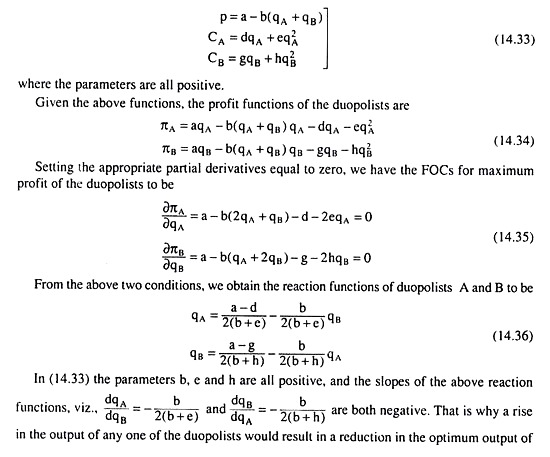
Let us now suppose that the market demand function for the product and the cost functions of the duopolists are:

Comparison between the Cournot Solution and the Quasi-Competitive Solution:

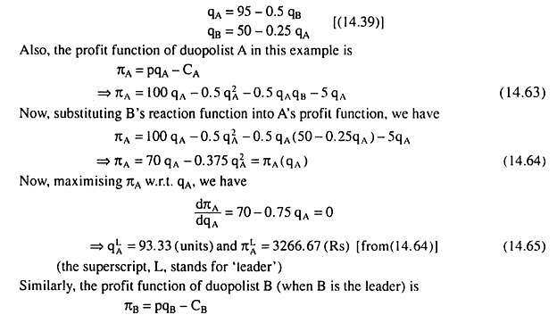
We may now compare the Cournot solution (14.37) with the quasi-competitive solution by using the example given in (14.5). The example gives us: a= 100, b = 0.5, d = 5, e = 0, g = 0and h = 0.5. Putting these values in (14.36) we obtain the Cournot reaction functions to be

If we now compare the Cournot solution (14.40) with the quasi-competitive solution (14.8), we find that the Cournot duopolists produce a smaller total output, sell at a higher price and earn larger profits.

The Output Leadership Model/The Stackelberg Model:

In this model, we shall retain the assumptions (i) to (ix) of the Cournot model, and the assumption (x) here would be:

(a) The duopolist A conjectures that B will accept A’s output as autonomously given and

(b) B will actually behave in this way.

That is, in this model, A is the output-leader and B the output-follower.

A is the leader because, he will choose the output which he will produce in the light of his correct conjectures about B’s reactions, and B is the follower because he will accept any output that A might produce as autonomously given.

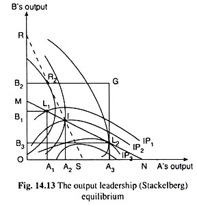
Given the assumptions (i) to (ix), the profit-indifference curves of the duopolists would be like those of the Cournot model. Some of these iso-profit curves have been drawn in Fig. 14.13. Assumption (x) implies that A knows B’s Cournot reaction function, for as we shall see, he would have to maximise profit subject to the constraint that he remains on B’s reaction function which is given by the line MN in Fig. 14.13.

This line, shows what would be B’s output at each given level of A’s output.

The points of intersection (and tangency) between this line and A’s profit indifference curves, viz., the points like L₁, I, and L₂, give us the alternative levels of profit that the duopolist A may earn at different levels of his output in combination with B’s output.

For example, at A’s output = OA₁, B’s output would be L₁A₁ and A would be on his iso-profit curve IP₁. Similarly, at A’s output of OA₂ and OA₃, A would be on the iso-profit curves IP₂ and IP₃.

It is easily seen in Fig. 14.13 that the output leader, A, would select that point on the follower B’s reaction function where this reaction function touches one of his (A’s) iso-profit curves, for, at this point here the point L₂, the output combination of A and B, viz., OA₃ of A’s output and L₂A₃ or OB₃ of B’s output, would take A to the lowest possible iso-profit curve or the highest possible level of profit.

It is clear from above that in this leadership model, the leader has no use of his own reaction curve, for he simply chooses that point on his rival’s reaction function where he achieves the maximum possible profit. There is, therefore, no path along which the leadership equilibrium is reached—rather the equilibrium point like L₂ may be pointed out instantaneously in Fig. 14.13.

We may now compare the equilibrium in this leadership model with that in the Cournot model. In Fig. 14.13, the dotted line RS is the Cournot reaction function of duopolist A, i.e., his output production would react along this line if he accepts the output of B as autonomously given. The point of intersection I of the Cournot reaction functions of the duopolists gives us the equilibrium in the Cournot model.

If we compare now the point I with the point L₂, we find that at I, the duopolist A lies on a higher iso-profit curve, i.e., on a lower profit level than at point L₂, and B lies on a lower iso-profit curve, i.e., on a higher profit level than at L₂.

In other words, the output leader A would prefer the leadership equilibrium to Cournot equilibrium, and the output follower B would prefer the Cournot equilibrium to the leadership equilibrium.

Now, if the leadership equilibrium as obtained above is to be maintained over a succession of periods, then the assumption (x) of the model would have to hold over these periods. Not only this, but also A would have to accept B’s present pattern of reaction as given by his reaction function MN, and B must remain ignorant of the fact that A knows his reaction function.

We may also note that if the duopolists are not satisfied with the present position, then each of them may seek to alter it to his advantage. For example, A may try to convince B, by threat or rumour, to accept a reaction curve that lies below the present one, viz., MN. Because, he may then move on to a still lower iso-profit curve giving him a higher level of profit.

On the other hand, if B suspects that A knows about his autonomous behaviour, he would try to convince A that he will react along a curve that lies above MN. If he succeeds in doing this, A would move on to a point of tangency on a higher iso-profit curve giving him a lower level of profit, and B would be able to move on to a lower iso-profit curve, giving him a higher level of profit.

Mathematical Presentation of the Output Leadership (Stackelberg) Model:

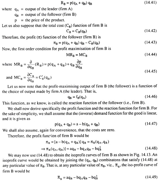
The follower (firm B) in the output leadership model wants to maximise profit. Let us suppose that the total revenue (R) function of the follower is

 

It follows from the properties of iso-profit curves that the profit of firm B will increase as it moves to the iso-profit curves further to the left (i.e., nearer the q_B-axis). That is why, at any particular q_A (output of firm A), firm B will produce that output (q_B) at which the ordinate at q_A would become a tangent to an iso-profit curve of B.

Therefore, at different values of q_A, we would obtain the corresponding values of q_B that would make the profit of firm B the maximum. If we join these (q_A, q_B) combinations by a curve, we would obtain the required reaction curve of firm B.

Since the demand curve for the product has been assumed to be linear, this reaction curve also would be linear like the line MN in Fig. 14.13. We have already obtained this reaction curve. It is given by equation (14.17).

This equation has been obtained by putting MR_B equal to zero (since MC_B has been assumed to be zero):

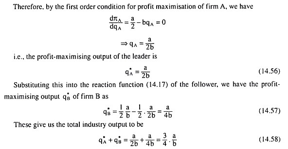
As we have already noted, the reaction curve of firm B, as given by eqn. (14.17), gives us the profit maximising output, q_B, of the follower (firm B) as a function of the given (and optimum) output, q_A, of the leader (firm A).

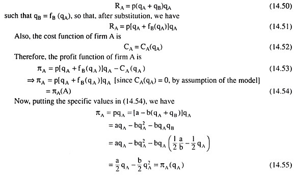
We have analysed above how the follower will choose his output given the choice of output of the leader. Let us now turn to the leader’s (firm A’s) profit-maximisation problem. By assumption (x) of the model, the leader is aware that his actions influence the output choice of the follower.

This relationship is summarised by the reaction function, q_B = f_B(q_A). Therefore, while determining his optimal output, he would recognise the influence that he would exert on the follower.

The profit-maximisation problem of the leader may be analysed, therefore, in the following way. The TR function of firm A is

Conjectural Variation and Stackelberg’s Analysis:

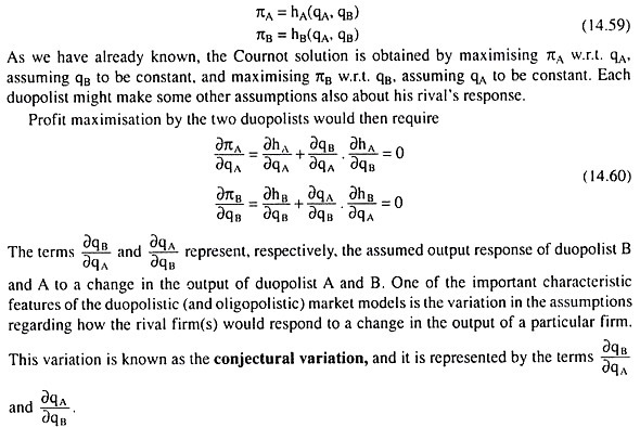
When there are only two sellers (firms) in the market for a product, we may assume that the profit of each seller is a function of the output levels of both:

An interesting example of conjectural variation is contained in Stackelberg’s analysis of leadership and followership. A follower obeys his reaction function given in (14.32) and adjusts his output level to maximise his profit, given the quantity decision of his rival, whom he accepts as a leader.

A leader does not obey his own reaction function. He assumes that his rival acts as a follower, and maximises his profit, given his rival’s reaction function. If the duopolist A desires to play the role of a leader, he assumes that B’s reaction function is valid and substitutes this relation into his profit function

π_A = h_A [q_A. Ѱ_B (q_A)]                               (14.61)

A’s profit now is a function of q_A alone, and can be maximised w.r.t. this single variable (q_A). Similarly, if the duopolist B wants to play the role of a leader, his profit function would be

π_B = h_B [q_B, Ѱ_A (q_B)]                                (14.62)

and he would have to maximise his profit w.r.t. the variable, q_B.

In this model, each duopolist determines his maximum profit level from both leadership and followership and desires to play the role which yields the larger maximum.

Four cases are possible here:

(i) A desires to be a leader, and B a follower;

(ii) B desires to be a leader, and A a follower;

(iii) Both desire to be followers; and

(iv) Both desire to be leaders.

As we have seen, case (i) results in a determinate equilibrium. Case (ii) would also result in a determinate equilibrium, since this case is the same as (i) with the two duopolists reversing their roles. Case (iii) also would have a determinate solution which is nothing but a Cournot solution under Stackelberg assumptions, since, here each seller acts autonomously, knowing that the other will also act autonomously.

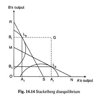
Lastly, in case (iv), both the duopolists aspire to be the leader. Here each assumes that he need not obey his reaction function, and rival’s behaviour is governed by his (the rival’s) reaction function. Thus, here neither of the reaction functions is obeyed, and we encounter a disequilibrium which is known as the Stackelberg disequilibrium.

Comparison between Stackelberg Solution and the Quasi-Competitive Solution:

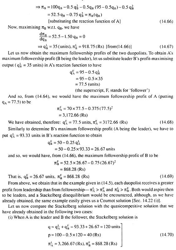
In order to compare the Stackelberg solution with the quasi-competitive solution, let us now go back to the example given by (14.5). We have already obtained the reaction functions of the two sellers to be

Here, as compared with the quasi-competitive solution, the Stackelberg duopolists produce a smaller output (120 < 190); sell it at a higher price (40 > 5); and the profits of both the sellers are higher (3.266.67, 868.28 > 0,12.5), and so their combined profit is also higher,

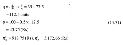
(ii) When B is the leader and A the follower, the Stackelberg solution is

Here also the Stackelberg duopolists produce a smaller output (112.5 < 190); sell it at a higher price (43.75 > 5); and the profits of both the sellers are higher (3,172.66, 918.75 > 0, 12.5), and so their combined profit is higher.

The Stackelberg Disequilibrium:

In this model, we shall suppose that both the duopolists are striving to be the output leader. We shall continue to make assumptions (i) to (ix) of the Cournot model. Our assumption (x), in this case, would be that each duopolist assumes that his rival would accept his output as given and constant, i.e., the rival would behave autonomously. In other words, each duopolist conjectures that his rival is an output-follower and he is an output-leader.

We may illustrate the consequences of these assumptions with the help of Fig. 14.14.

Let us suppose that initially A has been a monopolist and B suddenly joins the industry to compete with him. As per our assumption (x), A thinks that B would behave autonomously w.r.t. output, and he would react along his reaction function MN, and B also thinks that A would behave autonomously, and he (A) would react along his reaction function RS.

Under the circumstances, A would immediately accept the point L_a on the line MN as his profit-maximising point, and B would determine his profit-maximising position at the point L_b on the line RS, and, therefore, in period 1, A would produce the quantity OA_r of the product expecting B to produce OB, and B would produce OB_r of output assuming that A would produce OA₁.

That is, the combination of output that would be produced by the two firms in period 1 would be given by the point G (OA_r, OB_r) in Fig. 14.14. But G lies on a higher iso-profit curve in A’s map than the point L_a and it lies also on a higher iso-profit curve in B’s map than the point L_b, and so, both the duopolists would earn less than expected amount of profit in period 1.

Therefore, it would not be difficult for each of them to understand that his rival is not behaving as expected, and so, in the subsequent periods, each would seek some more appropriate conjecture about his rival’s reactions.

Each of them may go on experimenting and observing how his rival’s output plan reacts to changes in his own plan, or, each of them may desperately force his rival to react along some reaction function that suits him.

In the above analysis, we have seen that when each duopolist wants to become the leader, the hypothesis that each makes about his rival’s behaviour will be proved wrong.

However, the model helps us to understand what might follow from the given assumptions, and the assumptions, especially assumption (x), is not unrealistic. The model is also useful as it helps us to understand how and why the oligopolists may be driven to bargaining or collusion.