Let us discuss three topics related to factor payments. We first examine the pricing of fixed factors of production and the associated concepts of economic rent and quasi-rent.
We next examine some of the main factors which give rise to wage differentials.
Finally, we discuss the problem of factor shares in relation to the total value of the output of an economy, ‘the exhaustion’ problem, which has attracted the interest of economists for a long time.
A. Pricing of Fixed Factors: Rents and Quasi Rents:
1. Factors with Fixed Supply in the Long Run:
ADVERTISEMENTS:
We will examine the pricing of factors whose supply is fixed either in the short run or in the long run.
Fixed factors do not have a marginal product. Hence their price must be explained on different lines. The theory of pricing of fixed factors is based on the concept of economic rent. Economic rent is the payment to a factor over and above what is required to keep the factor in its current employment. In other words, economic rent is a payment to a factor in excess of its opportunity cost. If a factor has no alternative use its opportunity cost is zero; hence all its payment is rent.
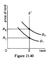
In the nineteenth century economists associated rent to the factor land. Later, however, the concept of rent was extended to all factors of production: any factor may receive an economic rent. The best example of economic rent is the payment to a factor whose supply is completely inelastic. For example the total area of land of a country, lakes, forests, mineral deposits are in fixed supply. The supply curve of such factors may be presented by a vertical line, such as the SS’ curve of figure 21.40; the available quantity of the factor is given irrespective of its price.
We may say that the price of a factor in fixed supply has no incentive function, in the sense that it cannot induce (give an incentive to) its owners to offer more of the factor as its price increases. As we will presently see, the price of the fixed factor has only an allocative role it ensures the use of the factor where it is most needed.
ADVERTISEMENTS:
When an input is in fixed supply its price is determined by the conditions of demand alone, since its supply is a constant quantity. For example assume that the land suitable for the production of grapes is OS (figure 21.40). If the demand for grapes gives rise to the demand curve Di for the grape-producing land the price of land (per unit) is However, assume that the demand for grapes increases; this shifts the demand for the particular land to D2. Given the perfectly fixed supply, the price of land increase to R2.
This change in the rent of land is solely due to the forces of demand. Under these conditions rent is not a cost entering in the determination of the price of grapes, but is the effect of the price of grapes, which, in turn, leads to a shift in the demand for the factor (land). In short, rent is price-determined, not price-determining, for the economy as a whole. For the individual firm (or farmer), however, all rents are costs, since the firm must pay such rents to the factors that create them in order to attract and keep these inputs, which otherwise would be bidden away by other firms in the industry.
If the fixed factor has no alternative use all its payment is rent the availability of the factor in its present use is not affected by whether its price is high or low. To state this in another way, if the factor has no alternative use its opportunity cost is zero, and nothing has to be paid to retain it in its present use. Hence, all payments to this factor is rent. It is clear that reducing (or taxing away) the payment to a fixed resource which has only one use does not affect its supply.
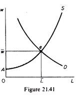
The return to a factor whose supply is completely fixed is often referred to as a pure economic rent. If the supply of a factor has some elasticity, part of its price is rent. To see that let us examine the market of a factor whose demand and supply curves are shown in figure 21.41. The equilibrium price is and the equilibrium quantity L.
The total payment to the factor is (0w) – (0L) = O Lew. This payment can be split in two parts the opportunity cost of the factor, that is the amount that must be paid to the factor to keep 0L units in their current use, and the rent of the factor, that is any payment in excess of the opportunity cost. We know that the supply curve shows the MC (marginal cost) of offering an additional unit of the factor.
Hence the amount required to keep 0L units in their current employment is the area OAeL. The remainder, Aew, is economic rent for the factor; it shows payment above what is required to keep each of the 0L units where it is currently employed. The economic rent, in this sense, is a surplus. Alfred Marshall called this economic rent ‘producer’s surplus’ it is a surplus return to the factor in excess of its opportunity cost.
It should be clear from the above discussion that any factor whose supply is less than perfectly elastic earns an economic rent. The steeper the supply curve of the factor, the greater is its economic rent. If the supply is perfectly elastic the factor payment contains no rent; it is all opportunity cost. If the supply is perfectly inelastic the entire payment to the factor is economic rent.
It is important to note that whether a payment is rent or not depends (a) on the elasticity of its supply, (b) on its alternative uses. Thus in each case we must be clear whether we are considering the supply of a factor to a firm, an industry or the economy as a whole. For example for the economy as a whole all land is paid a rent; its supply would not change if no price were paid. Consider next ‘agricultural land’, which refers to the supply of land to an ‘industry’.
Since agricultural land has alternative uses in other industries (e.g. housing construction), the price of agricultural land is partly rent and partly opportunity cost for the industry and the economy. In this event the supply of agricultural land would have a positive slope. The price of agricultural land paid by a single farmer, however, is opportunity cost. All rents are costs for individual producers.
It is important to know whether or not a certain payment to a factor is rent. Because if it is rent its reduction will not influence the supply and use of the factor. Whereas, if it is not a rent, a reduction in the payment is likely to change the allocation of the resource.
2. Factors with Fixed Supply in the Short Run:
In the short run some factors are fixed, while in the long run they become variable. The payment to an input which is in fixed supply in the short run is called quasi-rent, because it disappears in the long run (as the factor becomes variable), unlike rents which persist in the long run.
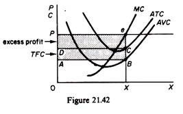
In the short run fixed inputs cannot be withdrawn from their present use and transferred to another where payments are higher, while variable inputs are free to move to alternative uses where returns are highest. Thus, firms pay the variable inputs their opportunity cost (otherwise these factors would move elsewhere), while the fixed inputs receive what is left over; quasi-rents are a residual payment. To understand this we examine the short-run equilibrium of a firm in a perfectly competitive market (figure 21.42). Assume the price is P. The firm maximises its profit, producing OX units of output, from which it receives a total revenue (TR) equal to the area OPeX.
The firm pays 0XBA = TVC to the variable factors. (It cannot pay less and keep them in its employment.) The fixed factors earn the residual ABeP, which is the quasi-rent. Thus
Quasi-rent = TR – TVC
The quasi-rent can be divided into two parts, the total fixed cost (area ABCD in figure 21.42) and excess (or pure) profit (DCeP). The TFC is the opportunity cost of the fixed factors, that is, the return that would have been earned if the fixed factors were utilized in their best alternative employment (e.g. by another firm in the same industry which pays higher returns on the fixed factors).
The excess profit is the difference between the quasi-rent and the TFC:
ADVERTISEMENTS:
Quasi-rent = TFC + excess Π
or
Excess Π = Quasi-rent – TFC
In the long run the quasi-rent becomes zero and the firm is in equilibrium, earning just normal profits. In summary, the price of a factor, whose supply is fixed in the long run, is called rent. The price of a factor, which is in fixed supply only in the short run, is called quasi-rent. Rent persists in the long run, whereas quasi-rent disappears in the long run as the factor becomes variable.
B. Non-Homogeneous Factors and Wage Differentials:
ADVERTISEMENTS:
We have assumed that factors are homogeneous. However, in the real world there are many different kinds of labour and each one commands a different price. The determination of the price of each kind of labour can be analysed within the general framework . We discuss briefly some of the factors that explain wage differentials for types of labour which are only partial (imperfect) substitutes for one another.
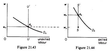
Let us first examine how wage differential arise. Assume that there are only two types of labour, skilled and unskilled, each with a perfectly inelastic supply curve. The market demand for each type of labour is the aggregate MRP curve, derived from the summation of theindividual firms’ marginal revenue product curves.
The two markets are shown in figures 21.43 and 21.44.
The supply of skilled labour is zero below the wage rate wu prevailing in the market of unskilled labour. If the wage for skilled labour is below wu nobody would be willing to undertake the cost and effort required to acquire the skills of the skilled market. The equilibrium wages are defined by the intersection of the demand and supply curves in each market. At equilibrium the wage differential between skilled and unskilled labour is wu ws.
The Causes of Wage Differentials can be classified in Four Groups:
ADVERTISEMENTS:
(a) Differences in the nature of the various occupations,
(b) Differences in the biological and acquired abilities of the various individuals which give rise to differences in their marginal productivities,
(c) Differences in the price of the output which labour produces,
(d) Market imperfections.
Differentials arising from the characteristics of the occupations are called compensating or equalizing differentials, because they represent payments made to equalize the net remuneration and compensate the workers for differences in their job.
Such Differences Arise from the Following Factors:
ADVERTISEMENTS:
1. Differences in the cost of training. Some occupations require large investments in training, while others require a much smaller expenditure for training. A physicist must spend eight years in undergraduate and graduate training. A surgeon may require ten or more years of training. During this period income is forgone and heavy educational costs must be incurred.
2. Differences in the costs of performing the job. For example dentists, psychologists and doctors in general require expensive equipment and incur high expenditures for running their practice. In order for net compensation to be equalized, such ‘workers’ must be paid more than others.
3. Differences in the degree of difficulty or unpleasantness of the work. For example miners work under unpleasant conditions relative to farmers.
4. Differences in the risk of the occupation. For example a racing driver or an airplane pilot run more risks than a college teacher.
5. Differences in the number of hours required for an ‘adequate’ practice. For example doctors are required to put longer hours in practising their profession than post office employees.
6. Differences in the stability of employment. Construction work and athletic coaching are subject to frequent layoffs and hence have little job security, whereas tenured university teachers have a high job security.
ADVERTISEMENTS:
7. Differences in the length of the employment. For example boxers and football players have a short working life.
8. Differences in the prestige of various jobs. For example a white-collar worker has a more prestigious position in society than a truck driver.
9. Differences in the environment. For example an engineer sent to Alaska or to a politically unstable African nation must be paid more than an engineer working in London.
10. Differences in the cost of living in various areas. Living costs generally are lower in small towns than in big cities.
Differentials in wages arise also from biological and acquired differences in the quality of labour offered by various people. These are called non-equalizing or non-compensating wage differentials because they are due to the differences in the marginal productivities of individuals.
Human beings are born with different abilities and in different environments, which define largely the opportunities to develop their inherent qualities. For example not many people are born with the biological qualities required for becoming successful tennis players or surgeons, writers or artists. And relatively few have the means and opportunities to develop themselves into tennis players or surgeons or artists. Biological and acquired quality differences among people are the major reasons why there are so many different wage rates even within the same occupation; the marginal productivities of workers differ.
ADVERTISEMENTS:
A major cause of wage differentials is the price of the commodities which labour produces. For example consider two hunters, the one hunting seals and the other hunting beavers. Both hunters are equally skilled, but the value of their output differs because the price of seal skins is higher than the price of beaver skins. In this case the difference in wages paid to the two individuals will equal the difference in the total value of their output.
Suppose that individual A (with the appropriate equipment and materials) produces an output with a value of £500 per week, while individual B (with the same equipment and materials) produces an output with a value of £450. In equilibrium the weekly wage of A would be £50 higher than that of B.
If the difference in wage was less than £50 an entrepreneur would replace B with A, since this would add to the value of output £50 and to costs less than £50. If the difference in wage was more than £50 the entrepreneur would replace A with B, since the decrease in the value of the output would be £50, but the decrease in costs would be more than £50.
Finally, wage differential arise from market imperfections. Imperfect knowledge of job opportunities may keep wages high in some regions. Immobility of labour may cause chronic unemployment and low wages in depressed areas. Labour unions, minimum-wage requirements and discrimination against minorities may also explain many wage differentials.
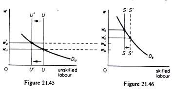
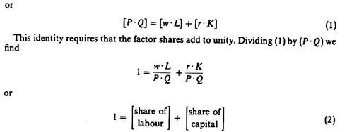
Wage differentials may widen or narrow over time. If the higher-paying jobs induce people to acquire the required skills, and if there are no union or professional bodies to bar entry in such jobs, wage differentials will tend to decrease. Referring to figures 21.45 and 21.46, the training of a larger number of previously unskilled labour, will shift the supply curve for skilled labour to the right and the supply curve for unskilled labour to the left.
These shifts will increase the wage of unskilled labour and decrease the wage of skilled labour, thus narrowing the wage differential to w’s w’u. Labour unions and professional bodies resist such equalisation movements. Labour union apprenticeship rules and the medical profession’s insistence on keeping down the enrolments in medical schools illustrate the forces which restrict entry to various occupations in an attempt to maintain or increase wage differentials.
On the other hand, government policy in granting more scholarships and students’ loans as well as in encouraging technical education tends to increase the supply of technicians and professionals. Such policies tend to narrow wage differentials or prevent them from becoming wider.
C. The ‘Adding-Up’ Problem: ‘Product Exhaustion’ Theorems:
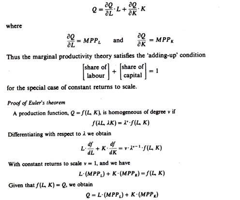
In the late 1930s considerable controversy surrounded the problem whether the factor prices, determined by the marginal productivity theory, would be such as to satisfy the basic ‘accounting’ identity
The value of the product must be exhausted by the factor payments. The question is whether the marginal productivity theory determines factor prices at the levels required to fulfil the basic ‘product = income’ identity.
The answer to this question is affirmative if the physical output is exhausted by paying each factor its marginal physical product, that is, if
Q = (MPPL). L + (MPP K). K (3)
Because: If we multiply through by P we obtain
PQ = (MPPL. P) L+ (MPPk . P) K (4)
But
(MPPL . P) = value of the marginal product of labour
(MPPk . P) = value of the marginal product of capital
and
PQ = value of output
Thus from (4) we see that if the factors are paid a price equal to their VMP, the total factor payments will exhaust the total value of the product, that is, the marginal productivity theory leads to the correct ‘adding-up’ of the factor shares.
1. Euler‘s ‘Product Exhaustion’ Theorem:
The mathematician Leonhard Euler proved that expression (3) holds for production functions which exhibit constant returns to scale (i.e. production functions
which are linear homogeneous). Euler’s theorem states that for a production function with constant returns to scale
Total physical (real) payments to factors would exhaust the total physical output.
Multiplying through by P, the price of output, we see that in the case of constant returns to scale that is, payment of factors according to their VMP exhausts the value of output, and share factors add up to unity.
PQ = L- (MPPL. P) + K. (MPPk. P)
Euler’s theorem is an identity it holds true for all values of the variables.
2. The Clark-Wicksteed-Walras ‘Product Exhaustion’ Theorem:
Clark, Wicksteed and Walras showed that the assumption of a homogeneous production function is not necessary for the fulfillment of the postulates of the marginal productivity theory. Their proof implies that, regardless of the production function, if factors are paid the value of their marginal physical product, then total factor payments will exactly exhaust the total value of the product in the long-run competitive equilibrium.
In the long run firms produce at the minimum point of their U-shaped LAC curve, and therefore the requirements of the Euler theorem hold. The Clark-Wicksteed-Walras proof is not an identity, since it holds only for the values of the variables in the long-run equilibrium.
Furthermore, it holds for all types of production functions, and hence it shows that product exhaustion is not a characteristic of the special case of the linear homogeneous production function. We present below a graphical proof of this theorem.
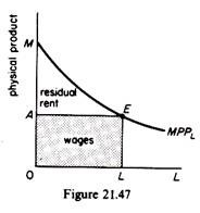
Assume that an economy consists of n identical firms. Figure 21.47 shows the product of a single firm.
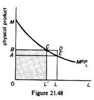
The MPPL curve shows the marginal physical product of labour. Assume that the firm employs 0L workers and a unit of land. The total product of each firm is the area 0MEL. If each worker is given his marginal physical product, then the ‘physical’ wage would be OA = LE and the total wages would be OAEL (shaded area in figure 21.47).
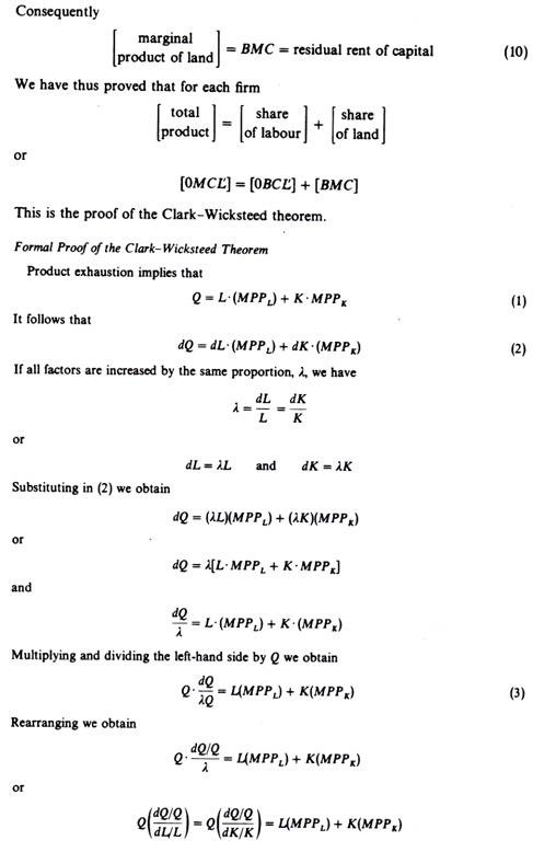
In other words the area OAEL is the total marginal physical product ‘paid’ to labour, or the share of labour (in physical units) in the total output of the firm. The remaining (physical) product AME is the rent of the fixed factor, land. We have to show that this residual rent is the total marginal product of land, that is, the share of land in output. With this proof we will establish the product exhaustion theorem.
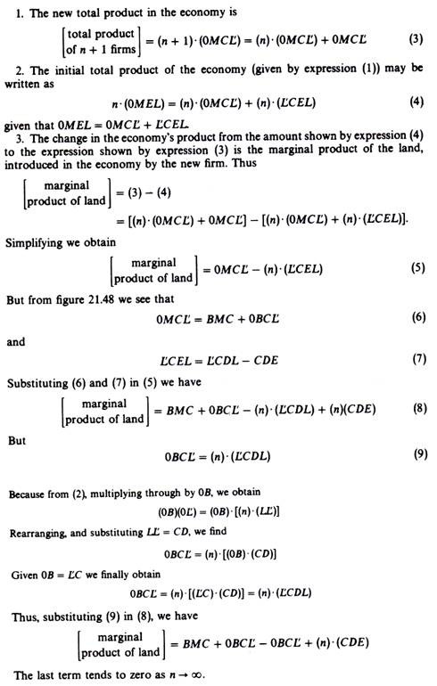
The total product in the economy is equal to the product of all n firms:
Assume that a new firm is added to the economy, having a plot of land identical to the land of the already existing firms, but not workers. For all the (n + 1) firms to be identical the total labour (n. (0L)) must be equally distributed between all of them. Thus each firm will employ less workers, say 0L, so that
(n+ 1)- (0L’) = n (0L) …(1)
and
0L = n- (0L — 0L) = n. (LL’) …(2)
The new output of each firm drops to 0MCL (figure 21.48). This consists of ‘physical wages’ 0BCL and a residual rent BMC. We will show that this residual rent is the share of land in the total output of the firm, so that the shares of the two factors exhaust the total product.
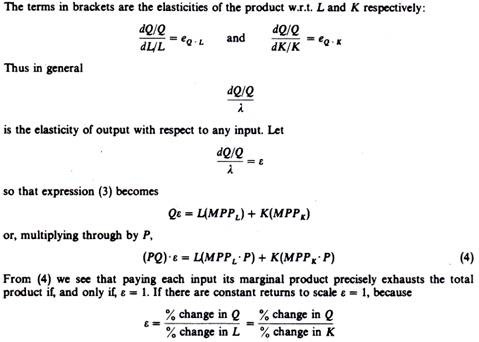
and the numerator (s) = denominators(s) when there are constant returns to scale.
Note that if ε = 1 (and there are constant returns to scale) the average cost is also constant. This is precisely what happens in the long-run equilibrium of a perfectly competitive firm the firm produces at the minimum point of its LAC. Thus the Clark-Wicksteed-Walras theorem holds only at the point of long-run competitive equilibrium; it does not hold for other values of the variables. In other words the Clark-Wicksteed-Walras proof renders the exhaustion expression (1) a theorem, not an identity holding for any set of values of the variables.
