Factor Pricing in Imperfectly Competitive Markets

The price of an input, when there are imperfections in the commodity and the actor markets, is determined by the same mechanism as in the case of perfectly competitive markets: demand and supply determine the price of the factor and the level of its employment.

However, the determinants of the demand and the supply are different in the case of market imperfections.

We will consider four models with various kinds of imperfections. In the first model we will assume that the firm has monopolistic power in the product market, while the factor market is perfectly competitive. We will next allow for imperfections in the demand for the factor.

In particular we will examine the case of a firm which has monopolistic power in the product market and monopsonistic power in the input market. The third model is the case of a bilateral monopoly the firm has monopson­istic power and the supply is controlled by labour unions. Finally the fourth model refers to the case of a firm which has no monopsonistic power and faces unionised labour supply. The above models are extensions of the marginal productivity theory of factor pricing and income distribution.

Model A. Monopolistic Power in the Product Market:

(a) Demand of a Monopolistic Firm for a Single Variable Factor:

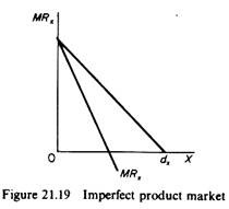
In this model we assume that the firm uses a single variable factor, labour, whose market is perfect the wage rate is given and the supply of labour to the individual firm is perfectly elastic. However, the firm has monopolistic power in the market of the commodity it produces. This implies that the demand for the product of the firm is downward-sloping and the marginal revenue is smaller than the price at all levels of output (figure 21.19).

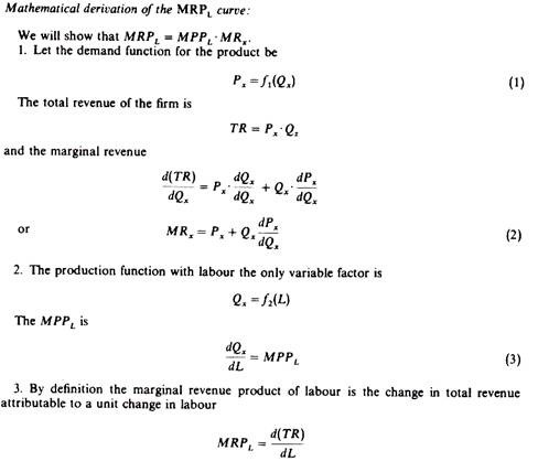
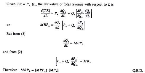
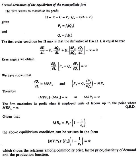
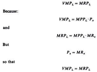
Under these conditions we will show that the demand for labour of an individual firm is not the VMP_L curve but the marginal-revenue-product curve, defined by multi­plying the MPP_L times the marginal revenue of selling the commodity produced

MRP_L = MPP_L. MR_x

We may illustrate the derivation of the marginal-revenue-product-of-labour curve.

The VMP_L (= MPP_L .P_X) is shown in column 8, and the MRP_L (= MPP_L MR_X) is shown in column 9. We observe that VMP_L > MRP_L. In figure 21.20 the VMP_L curve lies above the MRP_L curve at all levels of employment. This is due to the fact that P_x > MR_X at all levels of output and employment. Both the VMP_L and MRP_L have a negative slope because their components (MPP_L, P_x, and MR_X) decline as output expands and the price of the product falls.

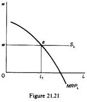
We will now show that the demand for labour is its marginal-revenue-product curve. Recall that in this model we assume that the labour market is perfectly competi­tive. Hence the supply of labour to the individual firm is perfectly elastic. This is shown by the horizontal line S_L in figure 21.21, which passes through the market wage w.

The firm, being a profit maximiser, will be in equilibrium at point e, employing l_i,units of labour. At this point

MRP_L = MC_L = w

In other words the firm is in equilibrium in the factor market when it employs units of labour up to the point where the marginal revenue product of labour is equal to its marginal cost. (Recall that MC_L = VP in a perfect labour market.) e is an equilibrium point because with employment I₁ the firm’s profit is maximised. To the left of e a unit of labour adds more to the revenue of the firm than the amount of its cost; hence it pays the firm to increase its employment.

Conversely at any point to the right of e an additional unit of labour adds more to total cost than to total revenue. Therefore, a profit-maximising firm (with monopolistic power in the product market) will employ labour up to the point where the marginal revenue product is equal to the wage rate.

The above analysis can be repeated for any given wage rate. Hence if only one variable factor is used, the marginal-revenue-product curve is the monopolist’s demand curve for this factor. In our numerical example the firm maximises its profit by employing six units of labour: at this level of employment MRP_L — w = £40 and total profits (£350) are at a maximum.

(b) Demand of a variable factor by a monopolistic firm when several factors are used:

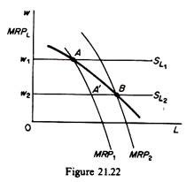
When more than one variable factor is used in the production process the demand for a variable factor is not its marginal-revenue-product curve, but is formed from points on shifting MRP curves. Suppose that the market price of labour is W₁ and that its marginal revenue product is given by MRP₁ (figure 21.22). The monopolistic firm is in equilibrium at point A, employing l₁ units of labour. If the wage rate falls to w₂ the firm would move along its MRP_L curve, to point A’, if other things remained equal.

However, other things do not remain equal. The fall in the wage rate has a substitution effect, an output effect and a profit-maximising effect, as in the case of a perfectly competitive firm. The net result of these effects is a shift of the marginal-revenue-product curve to the right (in general), which leads to the equilibrium point B. Generating points such as A and B at various levels of w we obtain the demand curve of labour.

Apparently the demand for a variable factor is more elastic when several variable inputs are used in the production process. We conclude that the demand curves for inputs are negatively sloped, irrespective of the conditions of competition in the product market.

(c) The market demand for and supply of labour:

The market demand for a factor is the summation of the demand curves of the individual monopolistic firms. In aggregating these curves, however, we must take into account their shift as the price of the factor falls as all monopolistic firms expand their output, the market price falls. The individual demand curves and mar­ginal revenue curves for the commodity produced shift to the left.

Graphically the derivation of the market demand curve for labour is exactly the same as that in figure 21.13 (p. 447), except that the individual demand curves are based on the marginal revenue product of the factor (and not on the value of the marginal product, as in the case of a perfectly competitive product market, where P_x is given for all firms). The market supply is not affected by the fact that firms have monopolistic power. Thus the market supply of labour is the summation of the supply curves of indivi­duals.

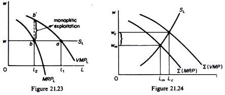
The market price of the factor is determined by the intersection of the market demand and the market supply. Thus the analysis does not change. However, there is an important difference the market demand is based on the MRP_L and not on the VMP_L. This means that when the firms have monopolistic power the factor is paid its MRP which is smaller than the VMP. This effect has been called monopolistic exploitation by Joan Robinson. It is shown in figure 21.23 for an individual firm, and in figure 21.24 for the labour market.

According to Joan Robinson a productive factor is exploited if it is paid a price less than the value of its marginal product (VMP). We saw that a profit maximiser will employ a factor until the point where an additional unit adds precisely the same amount to total cost and total revenue.

For a perfectly competitive firm:

Thus when the commodity market is perfectly competitive the profit maximising behaviour of firms leads to the payment of factor prices which are equal to the value of the marginal product (VMP) of the factors.

However, the condition of equilibrium of a monopolistic firm is:

MRP_L = MPP_L . MR_x = w

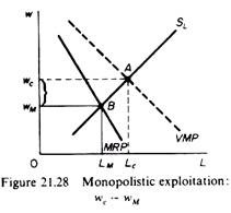
and MR_X < P_x, so that factors are paid less than the value of their marginal product. The difference bb’ in figure 21.23 and w_cw_m in figure 21.24 shows that profit- maximising behaviour of imperfectly competitive firms causes the factor price to be less than the value of its marginal product. Furthermore the level of employment is lower in industries which are not perfectly competitive (L_c > L_m).

Joan Robinson’s argument of ‘exploitation’ cannot be accepted on its face value. The fact that labour gets a lower wage in industries where competition is imperfect reflects the downward slope of the firms’ demand curve, which is due to the brand loyalty of consumers. Product differentiation reflects consumers’ desire for variety
consumers want to be able to choose among substitute products.

The consequence of this desire is a divergence between price and marginal revenue and a lower wage. The lower wage is thus the price that consumers must pay for having a variety of the same product, and cannot be considered as exploitation of labour by firms. Only if product differentiation is excessive, or is imposed on consumers by large corporations, one could accept the argument of labour exploitation in monopolistic markets.

Model B. The firm has monopolistic power in the commodity market and monopsonistic power in the factor market:

(a) Equilibrium of a monopsonist who uses a single variable factor:

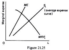
In this case the demand for labour by the individual firm is the same as in Model A. That is, the demand for labour by a monopolistic firm is the MRP_L. The supply of labour to the individual firm, however, is not perfectly elastic, because the firm is large. For simplicity we assume that the firm is a monopsonist (i.e. the only buyer) in the labour market. In this case the supply of labour has a positive slope: as the monopsonist expands the use of labour he must pay a higher wage (figure 21.25).

The supply of labour shows the average expenditure or price that the monopsonist must pay at different levels of employment. Multiplying this price of the input by the level of employment we find the total expenditure of the monopsonist for the input.

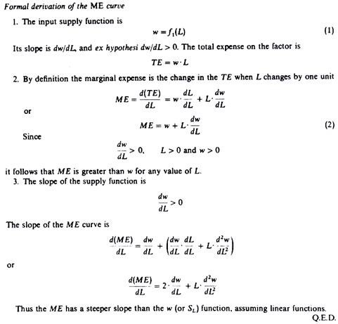
However, the relevant magnitude for the equilibrium of the monopson­ist is the marginal expenditure of purchasing an additional unit of the variable factor.The marginal expense is the change in the total expenditure (on the factor) arising from hiring an additional unit of the factor. Hiring an additional unit of input increases the total expenditure on the factor by more than the price of this unit because all previous units employed are paid the new higher price. Thus the marginal expense curve lies above the supply curve (or average expense curve).

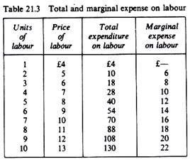
The marginal expense is the difference in the total expenditure at successively higher levels of employment of the factor. Table 21.3 illustrates the calculation of the marginal-expense-for-labour schedule. It is seen from table 21.3 that since the price per unit of input rises as employment increases, the marginal expense (ME) of the input is greater than its price at all levels of employment.

The ME curve has a positive slope and lies above and to the left of the supply of the input curve. This implies that the slope of the ME curve is greater than the slope of the supply curve, assuming linear relations.

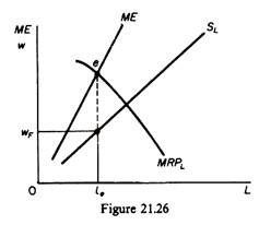
The firm is in equilibrium when it equates the marginal expenditure on the factor to its MRP. This is shown by point e in figure 21.26. The proof of the equilibrium is based on the definitions of the ME and MRP_L curves. At e the marginal expense (which is the marginal cost) of labour is equal to the marginal revenue product of labour. To the left of e a unit of labour adds more to the revenue than to the cost of the input; hence it pays the firm to hire additional units of labour.

To the right of e an additional unit of the factor costs more than the revenue it brings to the firm; hence the profit is decreased. It follows that profit is maximised by employing that quantity of labour (l_e in figure 21.26) for which the ME is equal to the marginal revenue of the input.

The wage rate that the firm will pay for the l_e units of labour is w_F, defined by the point on the supply curve corresponding to the equilibrium point e. To state this differently, w_F is the equilibrium wage corresponding to the equilibrium level of employment (l_e in figure 21.26). When the firm has monopsonist power in the input market it pays to the factor a price which is less (not only than its VMP, but also less) than its MRP. This gives rise to monopsonistic exploitation, which is something in addition to monopolistic exploi­tation. We saw that monopolistic exploitation arises from the fact that the demand for the commodity is negatively sloped so that MR_X < P_x.

The factor owners in this case are paid a price equal to the MRP of the factor, which is less than the factor’s VMP. Monopsonistic exploitation arises from the monopsonistic power of firms, and is something in addition to the monopolistic exploitation.

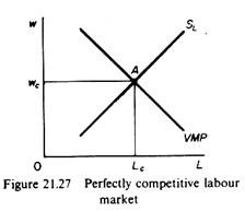
To illustrate this it is convenient to begin from the equilibrium wage rate when both the product and the factor markets are perfectly competitive. In figure 21.27 the VMP curve is the industry demand curve for labour and the S_L curve is the market supply of labour (free from any union activity). Demand and supply intersect at point A, and the equilibrium wage rate is w_c workers are paid the value of their marginal physical product (VMP).

Next assume that the commodity market is monopolistic, while the input market is perfectly competitive. The market demand for labour now is the MRP curve. It is the summation of shifting individual demand curves for labour. The labour market is in equilibrium at point B (figure 21.28).

The difference between w_c and w_M is the ‘mono­polistic exploitation’. Each unit of labour receives its MRP which is less than the VMP. Due to the monopoly power of firms, the price of the commodity will be higher and its demand lower. Hence the demand for labour will also be lower. Thus the result of ‘monopolistic exploitation’ is a lower wage rate and a lower level of employment.

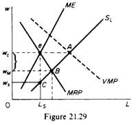
Finally, assume that the firm is a monopsonist in the labour market and a mono­polist in the product market. Its equilibrium is shown by point c in figure 21.29. The firm equates the ME of labour with its MRP (point e in figure 21.29). To maximise its profits the firm pays an even lower wage rate (w_s) and reduces further its employment (L_s). Monopsonistic exploitation is shown by the difference of the competitive wage and the monopsonistic wage, w_c. — w_s.

This can be split into two parts. The part w_cw_M is due to the monopoly power of the firm; it would exist even if the firm were not a monopsonist in the labour market; hence this part is not uniquely attributable to monopsonistic elements. However, the part w_sw_M is due to the monopsonistic power of the firm in the labour market. This power enables the firm to pay a wage rate lower than the MRP of labour.

In summary:

(a) In perfectly competitive markets the factor is paid its VMP.

(b) If the firm has monopolistic power in the product market but no power in the input market, the factor is paid its MRP < VMP.

(c) If the firm has both monopolistic power in the product market and monopson­istic power in the input market the factor is paid a price which is even lower than its MRP. This is the basic characteristic of monopsonistic exploitation. The input price is determined from the S_L curve so that the factor does not get its MRP, which is its contribution to the total receipts of the firm.

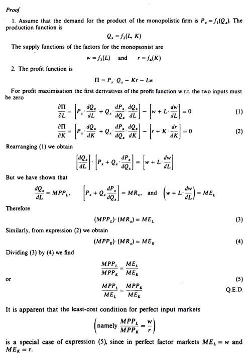
In the above analysis it was assumed that the market supply of labour is free from unionisation. This assumption will be relaxed in the model of bilateral monopoly. Let us now extend Model B to the case of a monopsonist who uses several variable factors.

(b) Equilibrium of a monopsonist who uses several variable factors:

If the input markets are perfectly competitive the firm minimizes its cost by using the factor combination at which

If the factor markets are monopsonistic, changes in the amount of factors employed causes changes in the prices of factors. Thus w and r are not given. The monopsonist must look at the marginal expense of the factors. It can be shown that a monopsonist who uses several variable factors will use the input combination at which the ratio of the mpp to the me is equal for all variable inputs. The least-cost combination is obtained when the marginal rate of technical substitution (mrts_{L . k}) equals the marginal expense of input ratio. For the two-input case the equilibrium condition of the monopsonist may be stated as follows

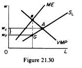
The size of monopsonistic exploitation depends on the structure of the commodity market. For example in figure 21.30 we show the case of a firm which is a monopsonist in the labour market, but sells its product in a perfectly competitive market. Equilibrium is attained at point G, and monopsonistic exploitation is the total difference w_c — w_F, since there is no ‘monopolistic exploitation’ in this case. Thus, the above diagrammatic analysis can be applied to all types of market organisations (all degrees of imperfections).

Model C. Bilateral monopoly:

In this model we assume that all firms are organised in a single body which acts like a monopsonist, while the labour is organised in a labour union which acts like a
monopolist. Thus we have a model in which the participants are two monopolies, one on the supply side and one on the demand side. In general bilateral monopoly arises when a single seller (monopolist) faces a single buyer (monopsonist). An example of a bilateral monopoly is the case of a single uranium mining company and the uranium miners’ union in a small town.

We will show that the solution to a bilateral monopoly situation is ‘indeterminate’. The model gives only upper and lower limits within which the wage rate will be determined by bargaining. The outcome of the bargaining cannot be known with certainty. It will depend on bargaining skills, political and economic power of the labour union and the firms, and on many other factors.

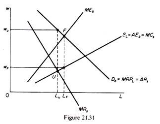
In figure 21.31 the monopsonists’ (single buyer’s) demand curve is D_b. It is the MRP_L of the input being demanded. From the point of view of the monopolist (labour union) this curve (D_b) represents his average revenue curve. Thus we denote this curve as D_b — AR_S (average revenue curve of seller). The seller’s (union’s) MR_S curve can be derived by the usual graphical technique; the MR_S will lie below the AR_S (and will cut any horizontal line at its mid-point).

The supply of labour facing the monopsonist is the upward sloping curve S_L. This shows the average expense (average cost) of labour to the monopsonist. Correspond­ing to this average cost curve is the ME curve. From the point of view of the monopolist (labour union) the curve S_L is its marginal cost. A monopolist does not have a supply curve. But, if it is assumed that the monopolist behaves as if his price were determined by forces outside his control (that is, if he behaves as if he were a perfectly competitive seller), then the mc_s curve may be considered his supply curve.

Given the above cost and revenue curves we can find the equilibrium position of each participant in the market. The monopsonist (federation of manufacturers or management of a firm) maximises his profit at point F, where his marginal expense on labour (ME_b) is equal to the marginal revenue product of labour. Thus the monopsonist will desire to hire L_F units of labour and pay a wage rate equal to w_F.

The monopolist (labour union), on the other hand, maximises his profit (gains) at point u, where his marginal cost is equal to his marginal revenue. Thus the monopo­list (union) will want to supply U, units of labour and receive a wage equal to w_u.

The price desired by the monopsonist (firm’s management) is the lower limit of
price, which can be realised only if he could force the monopolist-seller to act as a perfect competitor. The price desired by the monopolist-seller, w_u, is the upper limit price, which could be realised if he could force the monopsonist-buyer to act as a perfect competitor.

Since the price goals of the two monopolists cannot be realized, the price and quantity in the bilateral monopoly market are indeterminate. That is, economic analysis cannot provide a determinate solution to a bilateral monopoly market. The only result is the determination of upper and lower limits to the price. The level at which the price will be settled depends on the bargaining skills and power of the participants.

The power of each participant is determined by his ability to inflict losses to the opposite party and his ability to withstand losses inflicted by the opponent. Thus the possibility of a strike (by labour) or a lock-out (by firm), the financial position of the union and the firm, the general attitude of the public towards a possible strike or lock-out, and other factors play an important role in determining the bargaining power of the two monopolists.

The examination of the process of collective bargaining between unions and firms goes beyond the scope of this textbook. It requires an extensive knowledge of the institutional framework within which labour unions and business management oper­ate, as well as examination of the extensive body of literature on collective bargain­ing. References for the interested reader are included in the Bibliography.

Model D. Competitive buyer-firm versus monopoly union:

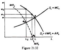
In this model it is assumed that firms have no monopsonistic or monopolistic power. The labour force, however, is unionised and behaves like a monopolist. The situation is shown in figure 21.32. The S_L curve shows the marginal cost to the union of supplying labour (as in the case of the bilateral monopoly). The market demand for labour curve D_L is the aggregate VMP_L curve, derived from the summation of the individual firms’ demand curves. This curve is also the average revenue curve for the union, from which the marginal revenue curve of the union, MR_S, is derived with the usual method. The wage in the market depends on the goal of the union. We will examine three of the most commonly pursued goals by labour unions.

(a) The Maximisation of Employment:

The highest level of employment is defined by the intersection of the demand and supply curves. Thus the union will demand a wage rate equal to w (in figure 21.32). The firms, being price takers, will maximise their profit by equating w to the VMP_L. Thus the total employment will be 0L.

(b) The Maximisation of the Total Wage Bill:

If the union aims at the maximisation of the total wage receipts it must seek to set the wage at the level at which the marginal revenue (to the union), MR_S, is zero. In this case the equilibrium of the union is at point e₁ (in figure 21.32). The union will set a wage equal to w₁ and the level of employment will be L₁.

(c) The Maximisation of the Total Gains to the Union as a Whole:

The attainment of this goal requires the union to set the wage at the level corresponding to the equality of the marginal cost and marginal revenue to the union. The equilibrium of the union is at point e₂ (in figure 21.32). The wage rate will be w₂ and the level of employment is L₂.

In summary, if the firms do not have monopsonistic power, the wage rate and the level of employment are determined by the goal of the union. It is interesting to examine whether labour unions are beneficial to their members. It is commonly believed that they are. In particular the effect of union activity depends on whether the firms have monopsonistic power and on the elasticity of the demand for labour.

1. Competitive Buyer-Firm versus Labour Union:

In the preceding paragraph we saw that the union can attain various goals. We will now examine whether the union members are better off when these goals are attained.

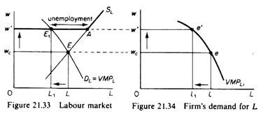
Figure 21.33 depicts the equilibrium of a perfectly competitive labour market. The market demand for labour is the aggregate VMP_L, and the supply of labour has a positive slope. The equilibrium wage rate is w_c and the level of employment is L. This is the maximum employment, given the profit-maximizing behaviour of firms.

Assume now that the labour force is unionised. What can the union do for its members? Apparently the union cannot increase the level of employment. Therefore the only alternative action is to seek an increase in the wage rate. The higher wage rate can be the total gain-maximising rate, the revenue-maximising wage, or some other compromise solution of higher wage and lower employment.

Assume that the union raises the wage rate to w’. The supply curve becomes the kinked curve w’AS_L in figure 21.33. That is, the union can make the supply of labour curve a horizontal line at the wage level that it sets, until the horizontal line reaches the initial supply curve. The new equilibrium of the firm is at e’ in figure 21.34, where w’ = VMP_L.

Thus each firm will reduce its demand for labour. The market equilib­rium is at the new intersection point E₁, (figure 21.33) of the demand and the new supply curve. Employment has decreased by the amount LL₁ and there is a total of E₁ A unemployed units of labour at the new wage rate.

In summary, the effect of the rise in the wage rate is a decline in the level of employment. The union members who lost their jobs are worse-off, unless the total wage bill has increased and the union distributes it equally between all its members (employed and unemployed). Whether the wage bill will increase following the rise in the wage rate depends on the elasticity of demand for labour.

If the demand is inelastic the union’s ability to increase the wage rate will increase the total wage receipts (wage bill) by the employed members. If the union redistributes these larger receipts to all its members, clearly the union’s action is beneficial.

However, if the demand for labour is elastic, not only the total employment but also the total wage bill will decline, and the union members as a whole will be worse off, although the ones who do not lose their job will be better off, because of the higher wage secured by the union. Thus when the firms have no monopsonistic power the effects of union actions are not necessarily beneficial to its members.

2. Monopsonistic Firm-Buyer versus Labour Union:

If the firms have monopsonistic power in the labour market a union can eliminate the portion of the total monopsonistic exploitation that is attributable uniquely to the monopsony power of the firm-buyers. A union can also increase the total wage bill, either by increasing the wage rate (but not beyond the level where the demand for labour is inelastic) or by increasing the level of employment or both. Let us examine these effects of union activity in some detail.

Assume for simplicity that there is only one firm-buyer in the labour market (monopsony). Since the labour is unionised we have the case of a bilateral monopoly. However, we will assume that the union does not attempt to maximise its gains. Instead we will examine two alternative goals, which, it is assumed, the unions can attain without leading to the indeterminacy of the pure bilateral monopoly model.

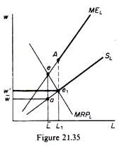
Assume that initially the labour is not unionised, so that equilibrium is attained at point e in figure 21.35, where the MRP_L is equal to the marginal expense of labour. The equilibrium wage is vv, and the equilibrium employment L.

Assume next that the workers create a labour union.

(a) The goal of the union is to maximise the level of employment. To attain this goal the union sets the wage rate at the level w’ (figure 21.35). The supply of labour is now the kinked curve w’e₁S_L, and the marginal expense curve is formed of two discontinuous segments w’e₁ and AME_L. The firm is in equilibrium at e₁, where MRP_L = ME_L.

Thus employment increases to L₁. Given that both the wage rate and the level of employment increase, the total wage bill increases (0w’e₁ L₁ > 0waL). Each worker receives a wage equal to its MRP_L; hence the exploitation attributable uniquely to monopsony is eliminated by the action of the union. However, the ‘monopolistic exploitation’ is not eliminated.

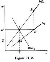
(b) The goal of the union is to obtain the maximum wage for the initial level of employment L For this the union sets the wage at the level w” (figure 21.36). The supply curve becomes the kinked curve w”eB’S_L and the corresponding ME_L consists of the two discontinuous sections w”eB’ and BME_L. The firm is in equilibrium at the initial point e, where the new ME_L is equal to the MRP_L. It pays w” as wage rate and employs L units of labour as in the pre-union period.

Thus w” is the maximum wage rate attainable without a reduction in the initial level of employment (L). The wage bill is obviously increased (0w”eL > 0WaL). Furthermore, the portion of monopson­istic exploitation attributable uniquely to the monopsony power of the firm is eli­minated, since w” = MRP_L. However, the ‘monopolistic exploitation’, attributable to the monopolistic power of the firm in the product market, is not eliminated.

(c) If the union attempts to set a wage rate higher than w”, employment will be reduced, and the total wage bill will depend on the elasticity of demand for labour. If the MRP_L curve is elastic the total wage bill will decline, while if the demand for labour is inelastic the wage bill will increase.

(d) Between the two extreme cases (a) and (b) the union can select intermediate policies, resulting in various increases in both employment and the wage rate.

The general conclusions emerge.

First:

If the firm-buyers have no monopsonistic power, labour unions can attain an increase in the wage rate at the expense of a lower employment. Whether this result is beneficial to all the members of the union depends on the elasticity of demand for labour and the distribution policies of the union.

Second:

If the firm-buyers have monopsonistic power, the union’s actions can eliminate one part of the monopsonistic exploitation, namely the part that is solely attributable to the monopsonistic power of the firms. However, the other portion of the monopsonistic exploitation, that which is due to the monopoly power of firms in the product market, cannot be eliminated by trade union action.

Third:

If the firm-buyers have monopsonistic power, trade unions can increase the total wage bill in most cases, by either increasing employment, or the wage rate, or both. Only if the demand for labour is elastic can the union harm its members, if it sets the wage rate above the maximum level for the initial (pre-union) level of employment.