Factors of Pricing in Perfectly Competitive Markets (With Diagram)

The mechanism of determination of factor prices does not differ fundamentally from that of prices of commodities.

Factor prices are determined in markets under the forces of demand and supply. The difference lies in the determinants of the demand and supply of productive resources.

In the nineteenth century economists classified factor inputs into four groups land, labour, capital and entrepreneurship.

The prices of these factors were called rent, wage, interest and profit respectively, and each one was examined by a separate body of theory. Since, however, there are many common factors underlying the determination of the price of inputs, a general framework can be developed for analyzing the price mechanism of any productive resource.

Thus, the theory to bedeveloped in will be presented in general terms, so that it is applicable to all factors of production. Given that labour is the most important input, we will usually speak of ‘the demand for labour’ or, ‘the supply of labour’. But the reader should interpret such expressions as implying ‘the demand for a productive factor’ and ‘the supply of a productive factor’.

We will first examine the determination of factor prices in perfectly competitive product and input markets. Subsequently we will relax the assumption of per­fectly competitive market and we will discuss factor pricing in markets with various degrees of imperfection.

A. Factor pricing in perfectly competitive markets:

In this part we will develop the so-called marginal productivity theory of distribu­tion. It takes its name from the fact that, in perfectly competitive product and input markets, factors are paid the value of their marginal physical product. The price of a factor, w, is determined by its total demand and supply schedules. The total demand is the sum (aggregate) of the demands of indivi­dual firms for the productive factor. Similarly, the total supply of a factor is the sum of the supplies by the individual owners of the factor.

We will develop the demand for labour by a single firm. The aggregate demand will then be derived from the summa­tion of the individual demands. The same approach will be adopted for the market supply. We will first derive the supply of labour by an individual consumer. The aggregate supply of labour will then be derived from the summation of the individual supply curves.

1. The Demand for Labour in Perfectly Competitive Markets:

We will examine the demand for labour in two cases:

(i) When labour is the only variable factor of production.

(ii) When there are several variable factors.

(i) Demand of a firm for a single variable factor

The following assumptions underlie our analysis:

(a) A single commodity X is produced in a perfectly competitive market. Hence P_x is given for all firms in the market.

(b) The goal of the firm is profit maximisation.

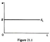
(c) There is a single variable factor, labour, whose market is perfectly competitive. Hence the price of labour services, is given for all firms. This implies that the supply of labour to the individual firm is perfectly elastic. It can be denoted by a straight line through w parallel to the horizontal axis (figure 21.1). At the going market wage rate the firm can employ (hire) any amount of labour it wants.

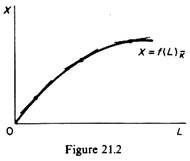
(d) Technology is given. The relevant production function is shown in figure 21.2. The slope of the production function is the marginal physical product of labour

dX /dL = MPP_L

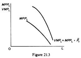
The MPP_L declines at higher levels of employment, given the law of variable propor­tions. If we multiply the MPP_L at each level of employment by the given price of the output, P_x, we obtain the value-of-marginal-product curve VMP_L (figure 21.3). This curve shows the value of the output produced by an additional unit of labour employed.

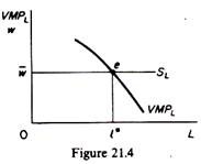
The firm, being a profit maximiser, will hire a factor as long as it adds more to total revenue than to total cost. Thus a firm will hire a resource up to the point at which the last unit contributes as much to total cost as to total revenue, because total profit cannot be further increased. In other words the condition of equilibrium of a profit maximiser in the labour market is

In figure 21.4 the equilibrium of the firm denoted by e. At the market wage rate w the firm will maximize its profit hiring l* units of labour. This is so because to the left of I* each unit of labour costs less than the value of its product (VMP_L > w), hence the profit of the firm will be increased by hiring more workers. Conversely to the right of l* the VMP_L < and hence profits are reduced. It follows that profits are at a maximum when VMP_L = w.

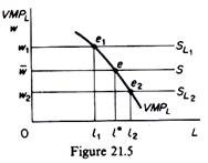
If the market wage is raised to w_1, the firm will reduce its demand for labour to l₁, (figure 21.5) in order to maximise its profit (at e_t in figure 21.5 w₁ = VMP_L). Si­milarly, if the wage falls to w₂, the firm will maximise its profit by increasing its employment to l₂.

It follows from the above analysis that the demand curve of a firm for a single variable factor is its value-of-marginal-product curve.

As an illustration of the above discussion consider the following numerical example.

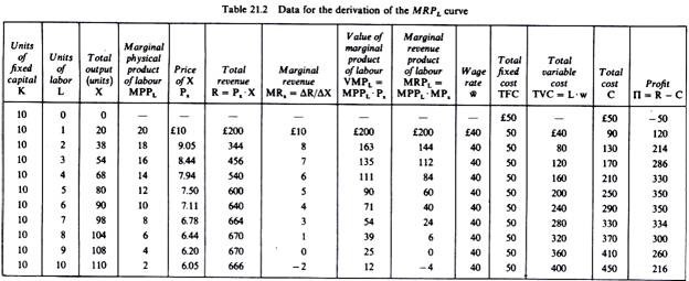
Assume a production process which involves a fixed amount of machinery (e.g. ten machines) giving rise to a total fixed cost of £50, and labour which is the only variable factor. The wage rate is £40 and the price of the commodity produced is £10. The production function is specified by the information of the first four columns of table 21.1. Column 6 shows total revenue (= X . P_x), column 10 includes total var­iable cost (=L. w). Finally column 12 shows the profit of the firm (∏ = R – TVC – FC).

The demand for labour which maximises the profit of the firm can be determined either by using the total revenue and total cost curves, or by using the VMP_L schedule and the given wage rate, which defines the supply of labour to the individual firm.

1. The Total Revenue-Total Cost Approach:

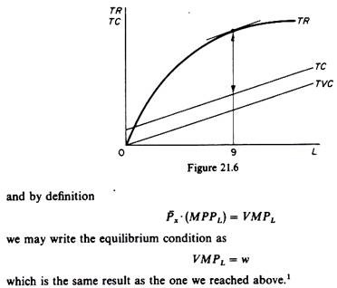
Profit is at a maximum when the difference between total revenue and total cost is greatest. In our example this occurs when nine units of labour are used. This solution, therefore, corresponds to the profit-maximising position of the firm. The total revenue-total cost approach is shown in figure 21.6. From this figure we see that the maximum distance between the two curves occurs when the firm employs nine units of labour. At this level of employment the slope of the total revenue and the total cost curves are equal.

The slope of the revenue curve is the marginal revenue per additional unit of labour, and the slope of the total cost curve is the wage rate, which in perfectly competitive markets is equal to the marginal cost of labour. Thus the condition for the equilibrium of the firm in the factor market is

2. The VMP_L approach:

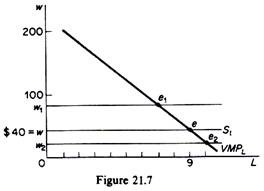
In figure 21.7 we show the VMP_L of our numerical example. The supply of labour to the individual firm is the straight line S₁ passing through the given wage rate of S40. The two curves intersect at point e, which defines the demand for labour (I = 9) at which the profit of the firm is at a maximum.

The firm is in equilibrium by equating the VMP_L to the market wage rate. If the market wage rises, the equality of w_t and VMP_L occurs to the left of e. Conversely if the wage rate falls to w₂ the equality with the VMP_L curve occurs to the right of e. Thus the value-of-marginal-product curve is the demand curve for labour of the individual firm.

(ii) Remand, of a Firm for Several Variable Factors:

When there are more than one variable factors of production the VMP curve of an input is not its demand curve. This is so because the various resources are used simultaneously in the production of goods so that a change in the price of one factor leads to changes in the employment (use) of the others. The latter, in turn, shifts the MPP curve of the input whose price initially changed.

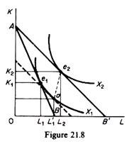
Assume that the wage rate falls. We will derive the new demand for labour, using isoquant analysis. The change in the wage rate has in general three effects: a substitution effect, an output effect, and a profit-maximising effect. Let us examine these effects, using figure 21.8.

Suppose that initially the firm produces the profit-maximising output with the combination of factors K₁, L₁, given the (initial) factor prices w₁ and r₁ whose ratio defines the slope of the isocost line AB. Now let us assume that the wage rate falls (w₂) so that the new isocost line is AB’ (the price of capital remains constant).

The firm, using the same expenditure, can now produce the higher output denoted by the isoquant X₂, using K₂ and L₂ amounts of capital and labour respectively. This result is derived from the tangency of the new isocost line AB’ with the highest isoquant, which, in our example, is X₂.

The movement from e₁ to e₂ can be split into two separate effects a substitution effect and an output effect.

To understand these two effects we draw an isocost line parallel to the new one (AB’) so that it reflects the new price ratio, but tangent to the old isoquant X₁. The tangency occurs at point a in figure 21.8. The movement from e, to a constitutes the substitution effect the firm will substitute the cheaper labour for the relatively more expensive capital, even if it were to produce the original level of output X₁.

Thus the employment of labour increases from L₁ to L₁. However, the firm will not stay at a. Because, when the wage falls, the firm, with the same total expenditure, can buy more of labour, more of capital, or more of both. Consequently the firm can produce the higher output X₂, employing K₂ of capital and L₂ of labour. The increase of employment from L₁ to L₂, corresponding to the movement from a to e₂, is the output effect.

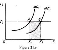
Point e₂ is not the final equilibrium of the firm. It would be if the firm were to spend the same amount of money as initially. However, keeping the total cost expen­diture constant does not maximise the profit of the firm. The firm will increase its expenditure and its output in order to maximise its profit. To understand this let us assume that the initial equilibrium of the firm is defined by point H in figure 21.9, where the firm’s MC is equal to the price of X.

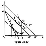
The fall in the wage rate shifts the MC curve downwards to the right, and the profit-maximising output of the perfectly competitive firm increases to X₃. This requires an increase in expenditures equal to the shaded area X₁ HGX₃. Thus in figure 21.8 the isocost line AB’ must shift outwards, parallel to itself, at a distance corresponding to the increase in the firm’s outlays. Actually the new isocost can be determined by dividing the increase (addi­tion) in total cost by the price of capital, r, and adding the result to the distance OA.

The new point, A’, on the vertical axis is the vertical intercept of the required isocost. The location of the firm’s new isocost curve is now determined, since this isocost is parallel to AB’. The final equilibrium of the firm will be denoted by the point of tangency of the new isocost A’B” with the isoquant denoting the profit-maximising output X* (point e₃ in figure 21.10).

In summary, the substitution effect of a decrease in the wage rate causes a decrease in the MPP_L because there is a smaller quantity of capital with which labour is com­bined. However, the output effect and the profit-maximising effect result in an increased employment of both inputs. Thus both these effects cause the MPP_L of labour to shift upwards to the right.

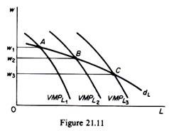
In general the output and profit-maximising effects more than offset the substitution effect, so that the final result of a fall in the wage rate is a shift of the MPP_L curve of labour to the right. Given the price of the final commodity, P_x, the VMP_L shifts to the right when several variable factors are used in the production process.

The shift is shown in figure 21.11. The new equilibrium demand for labour is denoted by point B on VMP_Lr By repeating the above analysis with different wage rates we can generate a series of points such as A and B. The locus of these points is the demand for labour by the firm when several factors are variable. This is sometimes referred to as the long-run demand for labour by the firm.

In summary, the demand of the firm for a single variable factor is its VMP curve. The demand for a factor when several resources are variable is the locus of points belong­ing to shifting VMP curves. This long-run demand for a factor is negatively sloped, because, on balance, the three effects of an input-price change must cause quantity demanded of the factor to vary inversely with price. Before we proceed further it is useful to summaries the determinants of the demand for a variable factor by an individual firm.

The demand for a variable factor depends on:

1. The price of the input. The higher the price of a factor, the smaller the demand for its services.

2. The marginal physical product of the factor, which is derived by the production function.

3. The price of the commodity produced by the factor. Recall that the VMP_L is the product of the MPP_L times the price of the commodity, P_x.

4. The amount of the other factors which are combined with labour. An increase in the collaborating factors will shift the MPP_L outwards to the right and hence will raise its VMP_L curve (and vice versa).

5. The prices of other factors, since these prices will determine their demand (and hence the demand for labour).

6. The technological progress. Technological progress changes the marginal phy­sical product of all inputs, and hence their demand.

(iii) The Market Demand for a Factor:

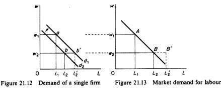
The demand curve of an individual firm for an ‘input. The next step is to use the demand curves of the individual firms in order to derive the market demand curve for the input. The market demand for an input is not the simple horizontal summation of the demand curves of individual firms. This is due to the fact that as the price of the input falls all firms will seek to employ more of this factor and expand their output. Thus the supply of the commodity shifts downwards to the right, leading to a fall in the price of the commodity, P_x.

Since this price is one of the components of the demand curves of the individual firms for the factor, these curves shift downward to the left. Figure 21.12 shows the demand curve d₁ of an individual firm for labour. Initially, suppose the wage rate is w₁. The firm is at point a on its demand curve and employs l₁ units of labour. Summing over all employing firms, we obtain the total demand for the input at the wage rate w₁. Point A in figure 21.13 is one point on the market demand curve for labour.

Assume next that the wage rate declines to w₂. Other things being equal, the firm would move along its demand curve d₁, to point b’, increasing the employed labour to l’₂. However, other things do not remain equal. When the wage rate falls, all firms tend to demand more labour, and the increased employment leads to an increase in total output. The market supply curve for the commodity produced shifts downward to the right, and the price of the commodity (given its demand) falls.

The decline in the price of the good reduces the value of the marginal product of labour at all levels of employment. In other words, the VMP_L curves (the individual demand curves for labour) shift downward. In figure 21.12 the new demand curve is d₂. When the wage rate falls to w₂ the firm is in equilibrium not at point b’ (on the original d₁ curve) but at point b on the new demand curve d₂.

Summing horizontally over all firms we obtain point B of the market demand curve. If the fall of the commodity-price was not taken into account, we would be led to an overestimation of the demand for labour following a decline in the wage rate. In figure 21.13 point B’ represents the demand for labour in the market with the price of the commodity unchanged. Note, however, that this point does not belong to the market demand curve for labour.

2. The Supply of Labour (A Variable Factor) in Perfectly Competitive Markets:

In this part we will concentrate on the derivation of the market supply of a variable factor. The most important variable factors are raw materials, intermediate goods and labour. The first two types are commodities, and hence their market supply is derived on the same principles as the supply of any commodity. The supply of labour, however, requires a different approach. To begin with we assume that labour is a homogeneous factor: all labour units are identical.

The main determinants of the market supply of labour are:

(a) The price of labour (wage rate).

(b) The tastes of consumers, which define their trade-off between leisure and work.

(c) The size of the population.

(d) The labour-force participation rate.

(e) The occupational, educational and geographic distribution of the labour force.

The relationship between the supply of labour and the wage rate defines the supply curve. The other determinants can be considered as shift factors of the supply curve. Since we are interested in the supply curve, we assume that all the other determinants are given (i.e. we make use of the ceteris paribus clause) in order to concentrate on the slope of the supply curve. The market supply is the summation of the supply of labour by individuals. Thus we begin by the derivation of the supply of labour by a single individual.

(i) The supply of labour by an individual:

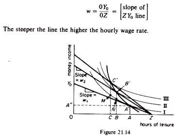
The supply of labour by an individual can be derived by indifference curves analysis. On the horizontal axis of figure 21.14 we measure the hours available for leisure (and work) over a given period of time. For example there are 0Z maximum hours in a day, which an individual can use for leisure or for work. On the vertical axis we measure money income. The slope of a line from Z to any point on the vertical axis represents the wage per hour. For example, if the individual were to work all the 0Z hours and earn a total income of 0Y₀, the wage rate would be

The indifference curves represent the preferences of the individual between leisure and income. For example on indifference curve II of figure 21.14 the individual is indifferent between OB hours of leisure and BZ hours of work (which bring to him an income of BN), and 0C hours of leisure and CZ hours of work (from which he earns an income of CM).

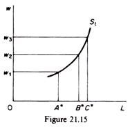
When the wage rate is w_t the individual is in equilibrium by working AZ hours, earning AA (= OA”) income and spending OA hours on leisure. If the wage rate increases to w₂ the individual will work more hours (BZ > AZ), will earn a higher income (BB’) and will have less hours (OB) for leisure. The supply of labour can be obtained from the locus of the equilibrium points A’, B, C’, etc. This supply curve is shown in figure 21.15.

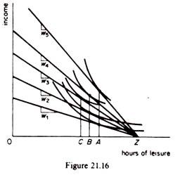
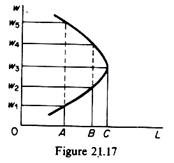
However, at some higher wage rate the hours offered for work may decline. For example in figure 21.16 if the wage rate is increased to w₄ the individual will work BZ hours, the same amount as when the wage rate was w₂.

If the wage rate increases still further (to w₅), the hours supplied for work decline even more they drop back to AZ. This pattern of response to higher wage rates produces a backward-bending supply curve for labour (figure 21.17).

Up to w₃, increases in wage rates create an incentive for increased supply of labour. However, higher wage rates create a disincentive for longer hours of work. The reason for this behaviour is the fact that longer working hours imply less leisure hours. As the wage rate increases, the individual’s income rises, and this enables the worker to have more leisure activities. However, the time for such activities is less. Hence beyond a certain level of the wage rate, the supply of labour decreases as r prefers to use his income on more leisure activities.

(ii) The Market Supply of Labour:

Although there is general agreement that the supply curve of labour by single individuals exhibits the backward-bending pattern, economists disagree as to the shape of the aggregate supply of labour. Several writers argue that in the short run the market supply of skilled labour may have segments with positive and segments with negative slope.

However, in the long run the supply must have a positive slope, since young people will be attracted to the markets where the wages are high and also older workers may undertake retraining and change jobs if the wage incentive is strong enough. Others maintain that the backward-bending supply curve of labour may be typical in most markets of the rich nations.

As the standard of living increases people find that unless they have the time to enjoy leisure activities it is not worth their while to work harder in order to obtain the higher income required for more leisure. Thus, as incomes reach the level required for a comfortable standard of living, workers put forward greater demands (in labour negotiations) for more holidays, longer vacations, shorter work weeks, fewer hours per working day rather than demanding ever higher wage rates associated with longer working hours. It seems that a positive aggregate supply of labour is the general case even for the affluent nations. Higher wages may induce some people less hours, but will also attract new workers in the market in the long run.

3. The Determination of the Factor Price in Perfect Markets:

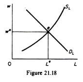
Given the market demand and the market supply of an input, its price is deter­mined by the intersection of these two curves.

In figure 21.18 the equilibrium wage is w^e and the employment level is L^e.

We see that the market model is valid for the determination of the equilibrium price of a commodity or a productive resource. The difference between commodity pricing and factor pricing lies in the determinants of the demand for variable factors and the method used to derive the supply of labour. The demand for factors is a derived demand, in the sense that the demand for the services of the factors is based on the demand of the commodities in whose production the factors are used. The supply of labour is not cost determined like the supply of commodities, but involves the attitudes of individuals toward work and leisure.