In this article we will discuss about the pricing of multiple and joint products.
The theory of price discrimination under monopoly can be extended to the problem of determining the prices for the multiple products of a firm. The extension of the theory was done by Eli W. Clemens. In reality, most firms produce more than one product. For this statement to hold good, two conditions must hold good.
First, resources of the firm be readily convertible to making a range of products, i.e., a major part of the equipment’s of the firm is general-purpose equipment and that management and labour are versatile. Second, the firm must have some idle capacity, i.e., the firm is not always locked in a rigid profit-maximising position. Writes D.S.
Watson, “With its idle capacity of plant, organisation, and personnel, the firm can expand production without having to expect much increase in marginal costs. Some of the idle capacity can be used to produce a second product for a second market provided that the demand in the second market is above marginal cost. More of the idle capacity can be put to work on a third product, a fourth, and so on.”
ADVERTISEMENTS:
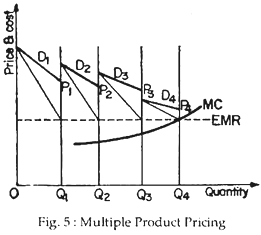
Fig. 5 here shows that the firm has four products that are sold in four markets. It lines the four markets up from left to right. The first market has demand D1, the second has demand D2, and so on. The quantity sold in the first market is OQ1; in the second market it is Q1Q2, and so on. The firm maximises its profits when it produces and sells quantities of each product such that their marginal revenues are equal to each other and equal to the marginal cost of total production.
Here, the line EMR is the line equal marginal revenue. So, we apply the equi-marginal principle here. In each of the four markets, the marginal revenue curves are the lines lying below the corresponding demand curves. The prices of the four products are shown in the figure.
Here, the fourth product has a price just above marginal cost. The more elastic its demand, the closer would the price of the last, or “marginal,” product to marginal cost. For part of its output, therefore, the multiple-product firm operates like the competitive firm, bringing one of its prices close to marginal cost.
ADVERTISEMENTS:
Since most firms produce more than one product they compete in several markets. For example, Philips India produces large radios (X2) and smaller transistors (X1). If the firm has a fixed amount of resources, it must allocate them between two products so as to maximise profit. Technology places constraints on the firm’s ability to substitute inputs.
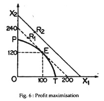
If more, radios are produced, fewer transistors can be produced. The product transformation curve in Fig.6 indicates the possible output combination given the fixed inputs. As resources are switched from transistors to radios, the tatter’s average productivity falls (or average cost increases).
Thus, the PPC is concave to the origin. The absolute slope is called the marginal rate of transformation—∆X2/∆X1. It increases as output moves to the right and decreases as it moves to left. The productivity of the inputs falls as they are concentrated on one product because not all of the firm’s factors of production are equally adaptable to the production of X1 and X2.
ADVERTISEMENTS:
The profit-maximising product mix can be found by the combing the production possibility constraint with profit function. Because the firm’s total cost for a given amount of resources is fixed, revenue maximisation is the same as profit maximisation. Let r1 be the price of a radio and r2 the price of a transistor.
The iso-revenue line is also shown here. It is a straight line because the competing firm can sell all it wishes at a given price. Any number of iso-revenue curve, such as R1 and R2, can be drawn. Each curve represents the same revenue produced by different combinations of the two outputs. The equation of the revenue line is R = r1X1 + r1X2 and its slope is r1/r2.
The optimal combination is determined by the tangency between the iso-revenue curve, R1 and the PPC. The firm cannot attain a higher revenue curve like R2 because of the production constraint. R1 is the highest revenue that the firm can reach and it should produce 100 units of X1 and 120 units of X2. At tangency (E), the negative slope of the iso-revenue, r1/r2, equals the slope of the marginal rate of transformation,
MRT = r1/r2 = – ∆X2/X1
A special kind of multi-product problem is joint product. An obvious example is pineapples and pineapple juice.

