Relationship between AC and AVC and between AC and MC

Let us learn about the relationship between Ac and AVC and between AC and MC.

First, AC = AFC + AVC

Second, AC = TC/Q

AVC is obtained by dividing the total variable cost by output, i.e., AVC = TVC/Q.

Thus, AVC is a part of AC, given AC = AFC + AVC. Furthermore, both the AVC and AC curves are U-shaped due to the operation of the law of variable proportions. However, the minimum point of the AC curve lies to the right of the minimum point of the AVC curve. (See. Fig. 3.20 where the point P—the minimum point of the AC curve—lies to the right of the point N—the minimum point of the AVC curve).

This is because AC not only includes AVC but also AFC which falls continuously as output rises. Not only this, initially, with the increase in output, AVC falls. So, AC must fall. AVC starts rising after OQ₁ output is being produced; its rise over a certain range is offset by a fall in AFC. That is why AC continues to fall over that range of output even if AVC rises.

That is why AC’s minimum point (point P) comes at a later range of output than AVC’s minimum point. Once OQ₂ level of output is produced the influence of a rise in AVC becomes stronger than the fall in AFC, so AC starts rising.

Now, we will establish a familiar relationship between MC and AC. We have said that MC is the change in total cost for a change in output.

Three points about the relationship between MC and AC are:

i. If MC < AC, then AC must be falling.

ii. If MC = AC, then AC is constant.

iii. If MC > AC, then AC is rising.

This relationship can be proved in this way:

MC = ∆(AC.Q)/∆Q, AC = TC/Q and, therefore, TC = AC.Q.

Thus, one obtains by substitution

MC = ∆ (AC.Q)/∆Q = ∆AC/∆Q.Q + AC (∆Q/∆Q)

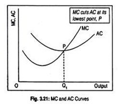
Since AC and Q are non-negative, MC > AC if and only if ∆AC/∆Q > 0. This means that AC increases with increase in output. Again, MC < AC, if and only if, ∆AC/∆Q < 0. This means that AC declines as output increases (Fig. 3.21).

This mathematical relationship can be established in terms of an example. Suppose, Sourav Ganguli scores 80 runs in the first innings of a Test Match and 90 runs in the second innings.

Thus, his average score becomes 85. If he scores 70 in the second match (let 80 to be the marginal score), his average score will now decline from 85 to 80. This means, when marginal score is less than average score, average score must be falling.

Notice that if MC < AC, then AC is falling. On the other hand, if he scores 85 in the second match then his marginal score (i.e., 85) will coincide with the average score. In terms of cost, when MC = AC then AC is constant. Finally, if Ganguli scores 100 runs in the next match (marginal score exceeds average score) his average score will now rise. Or whenever MC > AC, AC must be rising.

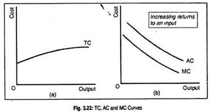
In this connection, it may be necessary to give reasons for the slopes of TC, AC and MC curves under various cost conditions. If we experience increasing returns to an input TC curve will look like Fig. 3.22(a).

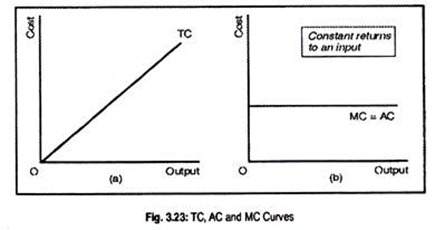
Since costs are diminishing due to the operation of increasing returns to an input, both AC and MC curves must be falling (see Fig. 3.23(b)]. On the other hand, if constant returns to an input prevail, TC curve will look like a 45° line while AC = MC curve will be parallel to the horizontal axis [see Fig. 3.23(a) and (b)].