In this article we will discuss about the Quantitative Analysis of Production Function with Cost.
Estimation of Production Function:
The production function is a technical relation showing how inputs are transformed into outputs. Three Inputs are usually considered: land, labour and capital. In Statistical (empirical) analysis, we often use man hours as the measurement of labour, machine-hours as the measurement for capital, and land-depletion as the measurement of land.
Output is defined as the finished products that are measured as a flow of goods and services during a given time period. The production function shows the maximum amount of output that a firm can produce for given amount of resources:
Q = ƒ(K, L etc.)…… (1)
ADVERTISEMENTS:
It may be added that the existence of a production function presupposes an optimum combination of inputs in the firm’s behaviour. The variables and parameters of the production function are independent of market prices of inputs and outputs.
Empirical Studies on Production Function:
Some empirical studies have already been made on the production function with a view to estimating its parameters. The data used in the estimation of the production function may be either a time-series or a cross-section sample.
Time-series data may contain a series of observations for outputs and inputs for a given firm or given industry over an extended period of time. K. J. Arrow, R. Dennison and others have argued that the state of technology is another important factor affecting the level of output.
In the long run, technological change may occur and technology may improve. Technological change has been most spectacular in the computer industry in recent years.
ADVERTISEMENTS:
In order to take account of technical change, one may include a time-trend in the production function as a proxy for measurement of such change:
Qt = ƒ(Kt, Lt,…, t)
Cross-section data can be obtained from individual firms or industries in a given period. The most common way is to collect output and input data from firms within an industry.
Without doubt the most celebrated production function is the Cobb-Douglas function. It owes part of its name to Professor Paul Douglas who, from empirical observations, inferred its properties, and part to his colleague Cobb, a mathematician, who suggested the mathematical form.
ADVERTISEMENTS:
The original formulation of the Cobb-Douglas production function is:
P = bLkCl–kU. (1)
where P is an index of total production per year, L is an index of labour inputs, C is the index of capital inputs, and U is an error term. The sample indexes were from 1899 to 1922, with 1899 = 100, as base. Cobb and Douglas argue that b, a constant, is independent of L and C.
The coefficient b is supposed to capture all those quantitative effects of any force for which they did not have quantitative data. The least squares technique was used to estimate the model. The results are
P = 1.0.1L3/4C1/4. (2)
Equation (2) indicates that for a 1% increase in labour input, with the amount of capital held constant, total output will increase by ¾ of 1%. By contrast, with a 1% increase in capital input and the amount of labour held constant, total output will increase by ¼ of 1%.
On the whole, if both labour and capital increase by 1%, the total output will increase by 1%. If interpreted in this way, the Cobb-Douglas production function has the property of constant returns to scale or homogeneity of degree one.
If we express the production function as
Q = AKαLβ (3)
ADVERTISEMENTS:
the degree of homogeneity is α + β, since
F(hK,hL) = A(hK)α(hL)β
= hα+βAKaLβ = hα+β Q.
Here, Q is output, A is a constant, K is capital input, L is labour input and α and β are two exponents of the production function.
Properties of Cobb-Douglas Production Function:
ADVERTISEMENTS:
1. We may note, at the outset, that in this functional form, both inputs are necessary to produce any output at all. If either capital or labour usage equals zero, output equals zero. That is, ƒ(K, 0) = ƒ(0, L) = 0. Furthermore, this form exhibits the required concave isoquant; so the MRTS will diminish.
2. For a Cobb-Douglas production function, the marginal products of capital and labour are, respectively
Since the marginal products must be positive, both α and β must be positive. The law of diminishing marginal product requires that the second derivatives be negative (i.e., Qkk and QLL must be negative). In this specification
ADVERTISEMENTS:
Thus, both α and β must be less than one. Combining these, we see that 0 < α, β< 1, i.e., marginal products are positive but decreasing. These marginal products are not constant but vary with the level of usage of the inputs. The marginal products have to be positive. In the context of Cobb-Douglas production function, the requirement is that α and β be positive. Furthermore, the law of diminishing marginal product requires, in this specification, that α and β be less than one.
Hence we need the following:
0 < α < 1 and 0 < β < 1.
The marginal rate of substitution of capital for labour is
ADVERTISEMENTS:
The Elasticity of Substitution:
One of the implications of the Cobb-Douglas production function is that factor rewards remain in fixed proportions. This distributional aspect of the function is summed up by a single parameter which is due to Hicks and is the elasticity of substitution. This determines (or is determined by) the shape of the isoquants and is defined as
To derive the elasticity of substitution we write this equation as
Thus, for the Cobb-Douglas production function the elasticity of substitution does not vary with the combination of factors used, and is equal to unity everywhere, so that a 10% change in relative factor prices brings about a 10% change in relative factor proportions. (Income distribution therefore, remains unchanged.)
ADVERTISEMENTS:
In other words, each parameter in equation (3) is also constant elasticity of output with respect to its input.
3. The Cobb-Douglas function has another property. It is a homothetic production function, which implies that it has a straight-line expansion path, i.e., changes in the level of output will have no effect on relative input usage (the ratio of labour to capital usage in the two-factor case).
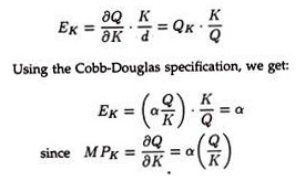
4. In a Cobb-Douglas production function, the coefficients α and β measure, respectively, the output elasticities of capital and labour.
The output elasticity of capital is
Likewise, the output elasticity of labour (EL) will equal β. 210ca075
ADVERTISEMENTS:
Using these coefficients, one can evaluate the impact of changes in capital or labour usage on output.
5. One important problem in the empirical analysis of a production function is to determine what happens to output when all inputs are increased proportionately. This situation comprises the returns- to-scale problem. There is some empirical evidence that production function for the economy as a whole approximates constant returns-to-scale. This particular function is called linear homogeneous production function.
The analysis of this particular form was summarized by Douglas. The sum of the exponents in the Cobb-Douglas production function shows the degree of returns to scale in production. Let us denote the percentage increase in input usage as k and the corresponding percentage increase in output as 1.
Then we can determine returns to scale by the following:
ADVERTISEMENTS:
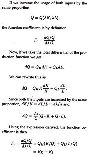
6. In a more quantitative manner, one can consider the question of returns to scale by considering a new measure called the function coefficient. Basically, this is a measure of elasticity since it reflects the percentage change in output in response to a given percentage change in the level of usage of both the inputs. We define the function coefficient, Fc, as
Fc = Percentage change in output/Percentage change in input usage
Thus, if there exists constant returns to scale, Fc = 1. If the production function exhibits increasing returns to scale, Fc > 1. In a like manner, if there exists decreasing returns to scale, Fc < 1. We may decompose function coefficient further. Since the increase in output is attributable to increases in the levels of usage of the individual inputs, it is possible to express it in terms of the inputs themselves.
For example, in the Cobb-Douglas case:
Hence, the function coefficient is equal to Fc = EK + EL.
That is, the function coefficient is equal to the sum of the two output elasticities.
This relation may now be demonstrated more explicitly. Consider the production function
Q = Q (K, L)
where EK and EL are again the output elasticities of A and L.
Therefore, in the case of our two-input Cobb- Douglas production function, the function coefficient is simply
Fc = α + β.
If α + β is greater than one, the production function is said to exhibit increasing returns to scale. Conversely, if α + β is less than one, decreasing returns to scale are observed. Finally, if α + β = 1 there is constant return to scale.
The Cobb-Douglas form will enable us to estimate the following:
1. Marginal products of the inputs.
2. Output elasticities.
3. Returns to scale.
In order to estimate this Cobb-Douglas production function, it is necessary to convert it into logarithms. Thus, the equation that will actually be estimated is
log Q = log A + α log A + β log L.
To see how such an estimation can be used, let us now turn to a few examples.
Example 1:
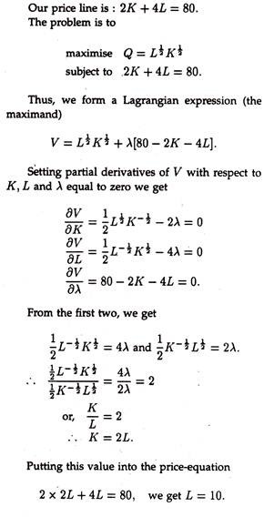
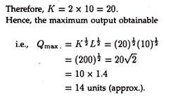
Given the production function Q = , L ½ K ½ and prices per unit of A and L is Rs. 2 and Rs. 4, respectively, and total cost of Rs. 80, determine the maximum output, subject to the cost constraint.
Solution:
Example 2:
Consider the production function:
Q = A- L0.6 K0.4
(Where Q is output, L, labour and K, capital)
Operate this function to estimate:
(a) The marginal rate of technical substitution,
(b) Elasticity of factor substitution.
Solution:
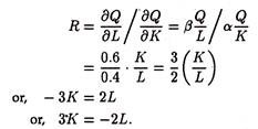
a) Here the marginal rate of substitution of capital for labour is
b) To derive the elasticity of factor substitution we write the above equation as
The CES Production Function:
Neoclassical economics emphasises the substitutability between factors of production, the ease of which is measured by the elasticity parameter a. The Cobb-Douglas function constrains a to equal one, which may or may not be a good approximation.
The constant elasticity of substitution (CES) production function also constrains the value of a to be constant, in the sense that it does not change with changes in relative prices or factor inputs. Its value is determined by the underlying technology and may change with technical progress, but in any event is not necessarily equal to one.
In the Cobb-Douglas case, under competitive conditions, the labour marginal productivity equation can be written as
Log (Q/L)= – log β + log (w/p)
and so output per head varies with the real wage rate (logarithmically) with a coefficient of unity. In contrast, Solow, Minhas, Arrow and Chenery (1961) —referred to as SMAC—observed cross-section regressions with a coefficient not equal to one
Log (Q/L)= α log b +log (w/p)
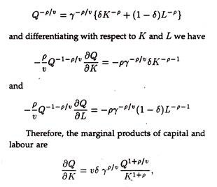
and derived the CES production function as a solution to this equation. The function is
Writing the right-hand side as F(K,L), then F(hK,hL) = hv F(K,L), and v gives the degree of homogeneity: in the original SMAC study v was taken equal to one and so constant returns were imposed. The parameter ϒ is a scale parameter which can be used to denote efficiency: a shift in ϒ is an example of neutral (neither capital nor labour saving) technical change.
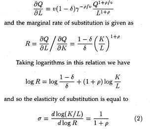
The degree to which technology is capital intensive is indicated by δ, and when the production function is embedded in a particular economic model δ can be interpreted as the distribution parameter. The substitution parameter p is equal to (1 —σ)/σ.
Rewriting the production function as:
and ranges from infinity (p = —1), which implies straight-line isoquants and perfect substitutability of factors, to zero (ρ = α) which implies rectangular isoquants and no substitutability of factors. This latter case corresponds to the Leontief’s input-output approach, and when ρ = 0, σ = 1, we have the Cobb-Douglas function.
(It can be shown that the CES production function reduces to the Cobb-Douglas production function as σ → 1, i.e., as ρ → 0)
Empirical work on this function has been carried out by a number of investigators using various estimation techniques. This has given rise to conflicting evidence about the elasticity of substitution, with some experts concluding that it is zero, some concluding that it lies between zero and unity and still others maintaining the view that the Cobb- Douglas function of unity best describes the data.
A major problem with the CES production function is that unlike the Cobb-Douglas, it is not possible to transform it into a linear-in-parameters form by operations such as taking logarithms.
The CES function admits the possibility of complementary factors rather than substitutable factors. If this is so then employment can only be increased in the short run if there is idle capital which can be activated as new labour appears. When all the capital is in use, employment cannot be further increased.
Uncertainty and the Production Function:
An important dimension often ignored in the theory of the firm is the role of randomness. However, some new models of production have been developed in recent years to take account of these elements.
Let us take the fixed coefficient type of production function which does not permit capital-labour substitution. There is no guarantee that the producer would get, when he hired an extra worker, the labour services he expected. The worker might fall sick. There may be a strike in the factory. Or, the labourer might turn out to be much more efficient than expected by the entrepreneur.
So, there are various sources of uncertainty. The producer can only think of a distribution of labour service and another of capital services, which he would get as a consequence of hiring fixed resources.
By doing this, he will find that the expected-output isoquants are smoothed out and he will be back in a neoclassical world with rounded corners to his isoquants. Such a smooth neo-classical function would relate inputs purchased to expected output.
Managerial Use of Production Functions:
1. The economics of production management takes, as its starting point, the study of the entire group of possible factor combinations that could be used to produce a certain output, within a given state of technology. This type of analysis is carried on through production function.
2. A production function is an expression of the dependent or functional relationship that exists between the inputs (factors) of a production process and the output (product) that results. Hence, it is sometimes known as ‘input-output’ relations.
3. Of the various types of production function, the C-D function is the most celebrated-, because it has certain important properties which are useful for managerial decision-taking as also for economic analysis.
4. The study of production function is useful not for its own sake but because it answers certain questions faced by management.
It enables management to know beforehand the most profitable decisions concerning the employment of resources and the scheduling of output. It is also useful in deriving a firm’s cost function.
For, once the physical relationship between a firm’s productive input services and its output are known (i.e., its production function), the firm’s cost function can be derived from the production function when the market prices of inputs (like rent, wage and interest rate) are given.
Short and Long Run Costs Estimation:
Various attempts have been made by economists and econometricians to estimate cost functions empirically. Empirical analysis of cost often deals with explicit accounting data regarding production cost. Such data are also used for cost analysis and control. Production costs are used for commodity pricing and output determination.
Any pricing decision is based on cost explicitly or implicitly. Any examination of the techniques of cost estimation is based on a new concept, viz., the cost function. So we have to introduce cost function at the outset. Different methods of estimation are used in case of different cost functions.
Brief Review of Cost Concepts:
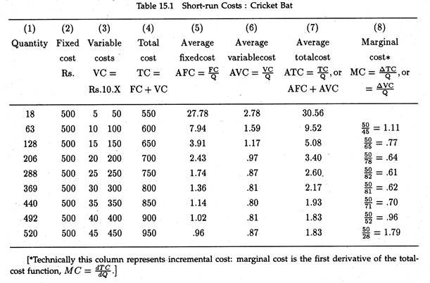
For decision-making purposes most firms rely on short-run, explicit costs. These costs are often expressed on a per-unit basis and are illustrated in Table 15.1 above on the basis of hypothetical date on the manufacture of cricket bat in a medium sized plant in Kashmir.
Here we illustrate the behaviour of costs in the short-run. So the production function from which the cost function is derived involves one fixed and one variable factor. Total fixed costs are Rs. 500.
We assume that the price (cost) of the variable factor remains unchanged at Rs. 10 per unit as output expands. If the costs of the variable factor were assumed to increase due to output expansion, the stage of (variable) diminishing returns to the input would be reached quickly. Consequently, both AVC and MC costs would increase sharply.
Average Variable Costs:
Average variable cost is total variable cost (TVC) divided by the level of output (Q). In Table 15.1, we observed that when output is 18 units, the AVC is Rs. 50/18 = Rs. 2.78. When output is 63 units, AVC = Rs. 100/63 = Rs. 1.59, and so on. Thus, AVC – TVC/Q.
It may alternatively be expressed as the reciprocal of average physical product, APP, multiplied by the average (unit) cost of the variable factor:
AVC = P (1/APP)
where P is the unit cost (price) of the variable cost. Suppose, for instance, APP — 3.6 and the price of the input is Rs. 10 per unit. Therefore, AVC is:
Rs.10 (1/3.6) = Rs.10 x .2773 = Rs.2.78
where Q — 18 units. This point can be verified by looking at column (6) of the above Table.
Since it is not possible to produce anything without incurring some costs, average costs are a reflection of average product. Conversely, AVC initially falls, reaches a minimum and rises subsequently. The curve, of APP and MPP reflect the law of diminishing returns. Since cost and productivity are the reciprocal of each other, AVC and MC curves are inversely related to the APP and MPP curves.
Average Fixed Cost:
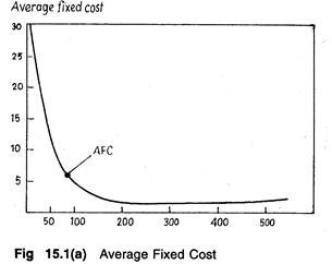
Average fixed cost (AFC) is fixed cost per unit of output. We arrive at AFC by dividing total fixed cost (TFC) by the quantity of output. Since TFC remains constant at levels of output up to capacity, AFC continues to fall as output increases, coming close to zero along the horizontal axis as in Fig. 15.1 (a) but never touching it.
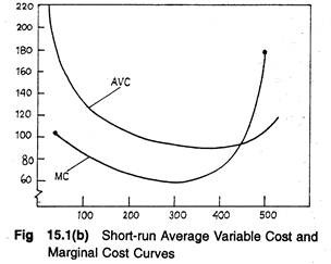
So the AFC curve is a rectangular hyperbola, i.e., it has a negative slope throughout. But AVC curve initially declines and reaches a minimum point and increases subsequently. This is because of the behaviour of total variable cost which initially increases less than proportionately, then more or less proportionately and finally more than proportionately as in Fig. 15.1(b).
Marginal Cost:
Marginal cost (MC) is the change in total cost associated with a finite (small) change in output. It is illustrated in column (8) of Table 15.1. In our example, MC is the amount by which TC changes when output moves in increments of 10 units. For continuous changes in output, MC is the first derivative of the total cost function (i.e., MC = dTc/dQ.
Since fixed cost remains constant at levels of output in the short run (when capacity is fixed) MC cost has no relation to fixed cost. In other words, MC reflects changes in variable cost associated with output changes. So, it is possible to calculate MC in Table 15.1 by noting changes in column 3.
Relating MC to the production theory, we calculate MC as follows:
MC = P(1/MPP) where MPP is the marginal physical product of the variable factor. In traditional text books it is expressed as:
MC = ∆TC/∆Q
for discrete changes in output. Here ∆ denotes any change.
A fundamental distinction between MC and AVC lies in their curvature in Fig. 15.1(a). AVC declines initially, then reaches its lowest point and finally increases in a gradual manner. On the contrary, MC curve responds fairly quickly to the law of diminishing returns.
In general, MC declines sharply, reaches its minimum and then subsequently rises sharply, intersecting the AVC curve at its lowest point and from the below. In Table 15.1, AVC is lowest (i.e., Re. 0.80) when Q – 440 units; MC reaches its minimum (i.e., Re. 0.61) much earlier, (i.e., when Q = 288).
Semi-fixed/Semi-variable Costs:
In theory, a distinction is always drawn between fixed cost and variable cost. But, in practice, this distinction often gets blurred. Therefore, members of a firm’s management team must reach a consensus in advance regarding specific definitions to be used by the firm for its fixed and variable cost allocation and production decisions.
Fixed costs, by definition, are those that do not change in the short run as output changes. In the long run, these costs cease to exist and all costs are treated as variable (because all factors of production, including the size of the plant or factory, is variable).
If this is our hypothetical cricket bat manufacturing firm, and if the firm has already spent (or committed) a specified sum of money for plant and equipment, wages, salaries, etc. and if this commitment is contractual and cannot be avoided for a fixed time period, the cost may be treated as ‘fixed’.
However, certain costs are partly fixed and partly variable in the short run such as telephone bill, wages and compensation of senior executives, certain labour and freight costs.
The most economic issues are negotiable. So, some items of fixed cost (like interest changes on external capital) are negotiable and hence avoidable even in the short run.
Variable costs, as the name suggests, do vary directly with the level of output, though not proportionately. Such costs exist in all time periods – short run and long run. Examples of short run variable costs are certain depreciation charges, some administrative charges, some labour costs, and other items reflected in a typical income statement (i.e., profit and loss account).
In the short run, for such costs, no contractual agreements exist inasmuch as such costs could not be negotiated and thus allowed to fluctuate upward or downward with changes in output. However, most of the examples cited under variable and fixed costs are neither variable not fixed in the true sense; instead they are semi-variable or semi-fixed.
In fact, a sharp distinction between fixed and variable costs is not always realistic. The managing director’s salary may be fixed for some purpose, but if the firm went into a really severe depression, this so called fixed cost could certainly be reduced.
In a like manner, the foreman’s wages might be fixed within a certain range of outputs, but, below a lower limit, foremen might be laid off (as in the U.S.A. where the hire-and-fire policy is adopted) while, above the upper limit, additional foremen would be hired. Again, the longer the duration of abnormal demand, the greater the likelihood that some fixed costs will actually be varied.
So the discovery that “certain costs are fixed only if output stays within prescribed limits, and that other costs can and will be varied if changed conditions are expected to persist, led to the development of the semi-variable cost concept. In incremental cost analysis, it is essential that one considers the possibility of semi-variable costs, which are fixed if incremental output does not exceed certain limits, but are variable outside these bounds.”
It is often assumed that variable costs are continuous functions of output when, in reality, some costs that remain fixed over considerable ranges of production increase by jumps, discontinuously, at various levels of output. Costs that exhibit this tendency have been classified as semi-variable (semi fixed) costs.
They consist of a fixed and variable portion, such as telephone expense, foremen’s wages, and certain owner expense elements which may remain constant for a wide range of output but then increases by definite jumps as output expands beyond certain limits.
This explains why members of the management group must decide and define in advance how much each cost incurred by the company will be treated for meaningful decisions relating to pricing and output.
The negotiation principle suggested that costs appearing as fixed can at times be made variable through successful negotiation. Many companies in the real commercial world survive by changing, via negotiations, fixed costs into variable ones.
Changes in Factor Productivities:
It is not difficult to see that productivities of factors of production are liable to change through time. For example, machines and equipment can be expected to become more efficient with the passage of time. This is due to technological progress.
A given amount of (real) investment in machines and equipment can be expected to yield a greater flow of output per period of ten years from now than they do today. Technical advances can, of course, be of various types. First of all, they can either be exogenous or endogenous in character.
When factors of production automatically become more efficient with the passage of time and there is no internal explanation of the technical advance, the technological progress is said to be exogenous.
On the other hand, when the economic model at hand explains the mechanism by which technological progress is generated, we have the case of endogenous technological progress. Exogenous progress, in its turn, can be of two types.
When it is embodied in new machines only, i.e., when with the passage of time we get more output (per unit of investment) out of the newly installed machines only (and the old machines retain their old levels of efficiency), the technological progress is said to be of the embodied type.
On the other hand, when all the factors of production (irrespective of their vintage) become more efficient with the passage of time, the exogenous technological progress is said to be of the disembodied type.
It is not relevant for our purposes here to examine which of these different notions of technological progress is most realistic. All that matters for us is that whenever technical advancement of any type occurs, the production function changes since we get more output out of the same level of (some of the) inputs.
It would be wrong to think that technical advancement affects the productivity of machines and equipment only. As people get more educated and more adopt at handling machines, productivity of labour inputs also increases.
The different types of technological progress that we have mentioned in the previous paragraph represent a general typology. Although people usually visualise technological progress in the form of newer machines, in economics we talk of technological progress whenever the efficiency of any factor of production increases.
With the passage of time, therefore, the cost function changes, since a cost function is derived from the production function. From the point of view of cost forecasting, a crucial task is to predict the rate of technological progress.
This is not a particularly difficult task. Often, one can observe the trend rate of technical advancement that has occurred in the past and predict the rate of future technical progress by extrapolating this trend.
One matter of detail is that official data regarding factor productivities are usually available in the form of average productivity of labour, i.e., the level of output divided by the amount of labour. Since output is actually the joint effect of labour as well as the other factors of production, this, in effect, an overall measure of technical progress.
If there is an upward trend in the data on average product of labour, the inference should not be that it is only labour that is becoming more efficient. If we keep this point in mind, the method of extrapolating labour productivity trends will provide us with a fairly dependable estimate of the rate of technological progress.
If a cost function has already been estimated on the basis of a given production function we can predict future costs on the basis of these predicted changes in the production function.
Changes in Factor Prices:
The other major source of changes in the cost function is the change in factor prices. If, say, due to inflation all factor prices change in the same proportion, the optimal factor combination for the company will remain unchanged. It will employ the same amounts of the different factors of production. However, since the price of each factor has changed, the total cost of production will change.
If, on the other hand, inflation affects the different input prices unequally, the total cost of production will change on two counts:
(1) The optimal factor combination for the company will change now. The company will use more of the factor whose price has risen relatively slowly and less of the factor whose price has risen more sharply. Since amounts of factors employed change, the total cost of production for the company will change.
(2) The cost of production will continue to be affected directly by the rise in input prices.
The change in the cost function caused by changes in factor prices can be predicted if we can form an idea about the rate at which prices of the different factors of production are going to change in the future. Opinion surveys, trend projections, econometric models, barometric indicators and related methods can be used for this purpose.
Again, since most of these methods were discussed at length in connection with demand forecasting, the reader will easily be able to see how to adopt them to the task of predicting changes in the price level.
Finally, the two set of information, those relating to changes in factor productivity and to changes in factor prices, have to be combined in order to arrive at a tolerably accurate estimate of future costs of production.
In a mass production system it is usually observed that as the cumulative volume of output increases, the quantity of factor inputs (like labour, capital etc.) required to produce each unit of output decreases. This, in its turn, leads to a fall in unit cost of production.
This phenomenon is known as the learning curve effect and is usually observed in the behaviour of labour inputs and costs. Various factors explain why the number of working hours required to produce each unit of output declines as more units of the product are produced.
The following factors are important:
(1) Familiarization with the tasks of workers and supervisors,
(2) Improvements in work methods and the flow of works,
(3) Reductions in the amount of scrap and reworks and
(4) The need for fewer skilled workers as the task becomes more repetitive.
Raw materials costs per unit may also fall due to learning effect as workers become more familiar with the production process.


