In this article we will discuss about the segments of production possibility curve showing production.
On a production possibility curve, segments are found only when the products are complementary or supplementary in nature.
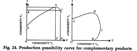
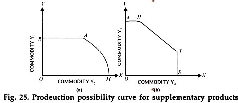
We have seen in Fig. 24 (b) as well as in Fig. 25 (b) that over segments AH and BT of the production possibility curve, the products are complementary or supplementary and over the segment HT, they are competitive.
Now, segments AH and BT of the production possibility curves in Fig. 24 (b) and Fig. 25 (b) are segments of irrational production. This is because whatever be the price of Y1 or Y2 movement from A towards H and from B towards T will increase the total revenue. So the farmer must move into the segment HT if he has to maximize his profits.
ADVERTISEMENTS:
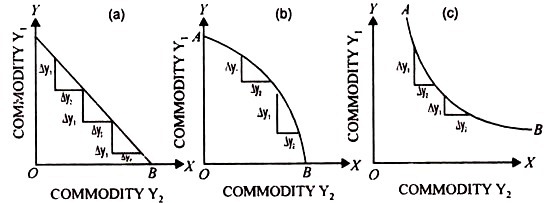
Where the point of maximum revenue actually lies, will depend upon the prices of the two products namely Y1 & Y2 But it will definitely lie between H & T i.e., in that segment of the production possibility curve where the two products become competitive. We may note here that in Fig. 23, the two products are competitive throughout. Each of three production possibility curves in that diagram thus contains only the stage of rational production.
Fig. 23. Production possibility curve for Completive Products
The Iso-revenue lines:
For determining the combination of two products, produced by using a given amount of an input as will ensure the maximum revenue, we need another tool of analysis.
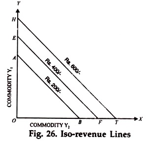
This is called an iso-revenue line. Just as a production possibility curve indicates various combinations of two products that can be produced by using the same amount of the variable input (x1), an iso-revenue line shows all possible combinations of two products which would yield the same total revenue.
An iso-revenue line for any total revenue can be easily draw by determining the extreme points on the axes of coordinates and connecting these points with a straight line. In Fig. 26, the pint on Y-axis is determined by the value TR/PY1 and that on the X-axis is determined by the value TR/ PY2. These points, in other words, show the amount of Y1 and Y2 respectively, needed to earn the given level of total revenue.
Fig. 26 shows three such iso-revenue lines, namely AB, EF and HT, representing three different levels of total revenue received by the production of two products Y1 and Y2 We may note here that a higher iso-revenue line will imply a higher total revenue, As such, EF represents a higher total revenue as compared to AB and will be parallel to AB if the prices of Y1 and Y2 are unchanged. Similarly HT will show a higher total revenue as compared with both EF and AB.
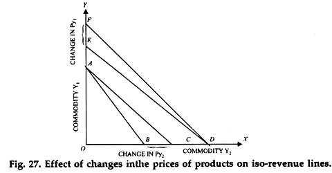
It is obvious that the slope of the iso-revenue line change if there is change in the relative prices of the two products Y1 and Y2as shown in Fig. 27. Suppose AE is the original iso-revenue line. Further suppose that the price of Y2 falls while the price of Y1 remain at the same level.
It is obvious that for earning the same amount of revenue, a larger quantity of Y2 say, OC (>OB) will have to be sold now when its price has fallen. However, as price of Y1 remains the same, the same quantity of Y1 will be required to be sold in order to earn the old revenue.
Thus a Shift in iso-revenue line from AB to AC in the diagram, is due to the decline in price of Y2. Similarly, a shift in the iso-revenue line from DE to DF in the diagram will take place when the price of Y1 falls while that of Y2 remains the same.
