Products and Production Possibility Curve

In this article we will discuss about the relationship between products and production possibility curve.

1. Joint Products with Fixed Proportions:

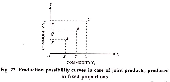
Products which result from the same production process are called joint products. In other words, the two products are so related to each other that the production of one automatically leads to the production of other.

The quantity of one product produced determines the quantity of the other product. In other words, the two products are always produced in fixed proportions. Production possibility curves for such joint products are shown in Fig. 22. Each level of the variable input gives rise to a production possibility curve which is represented by a single point only.

For production decisions, such products can be treated as one. Example of such products are wool and mutton, beef and cow hides or wheat and chaff.

(ii) Competitive Products:

Products are competitive when an increase in the production of one can be had only by reducing the output of the other product, given a particular level of variable resources. Such products compete for the same inputs at the same time.

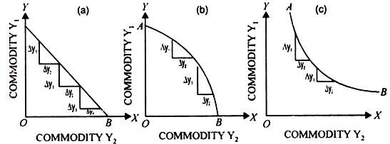
When two products are competitive, they may be transformed (or substituted) at constant rate, increasing rate or decreasing rate. The production possibility curve, though moving downwards to the right will have a different curvature in each of these situations as is shown in Fig. 23.

Fig. 23. Production possibility curve for Completive Products

In Fig. 23 (a) products substitute at a constant rate. As the production of Y₂ is increased, the output of Y₁ decreases by the same amount. In other words, the marginal rate of product substitution remains constant.

To express it in algebraic form we can say that in the direction of X-axis.

The production possibility curve in this case will be a straight line.

In Fig. 23 (b) substitution between two commodities is at an increasing rate. As each additional unit product Y₂ is produced, an increasingly greater sacrifice has to be made in terms of units of product Y₁ .The production – possibility curve, in this case, is concave to the origin. The algebraic form, this tendency will be expressed as follows in the direction of X-axis.

A production possibility curve concave to the origin will emerge when the law of diminishing marginal returns to the variable factor is operating in case of both the products or when the marginal returns to the variable input are constant in case of one product and are decreasing in the case of the other. The marginal rate of transformation is such a case is said to be increasing.

In Fig. 23 (c) marginal rate of product substitution is decreasing. As the output of product Y₂ is increased, the rate at which the output of product Y₁ is curtailed, steadily slows down. The production possibility curve, in this case, is convex towards the origin.

The decreasing rate of substitution between two products Y₁ and Y₂ is algebraically expressed as below: in the direction of X-axis.

We can come across a production possibility curve, convex to the origin when:

(a) The production of both the products follows the law of increasing marginal returns to the variable input or

(b) When the production of one product follows the law of increasing marginal returns to the variable input, the production of the other follows the law of constant marginal returns to the variable input.

In actual practice, it is generally the increasing rate of substitution which applies to competitive products because of the operation of the law of diminishing marginal returns. In other words the production possibility curve is generally concave to the origin.

(iii) Complementary Products:

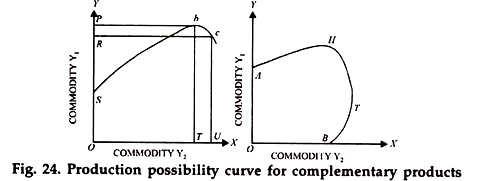
Two products say, Y₁ and Y₂ are complementary if inputs used to bring about an increase in the output of say product Y₁ also lead to an increase in the output of products Y₂ though not in the same proportion throughout. Production possibility curve in such a case is shown in Fig. 24.

Fig. 24 (a) gives only one extreme of the production possibility curve for a given amount of an input. But complementarity, if it exists, is experienced for both extremes of the production possibility curve as is shown in Fig. 24 (b). In Fig. 24 (b), H. and T represent maximum output level of Y₁ and Y₂ respectively with a given amount of an input.

Over the segments AH and BT, the products Y₁ and Y₂ are complementary as increased production of one product raises the output of the other product also whereas over the segment HT, they became competitive because the output of one can be raised only be reducing the output of the other. The complementary effects operate up to certain limits only. Competition between two products, then, is resumed as shown in Fig. 24 ‘(b).

In Fig. 24 (a) products Y₁ and Y₂ are complementary up to point b for a given amount of input. It may be noted at the two products cannot remain complementary to each other at all levels of production. After a point, increase in the amount of one will bring about a decrease in the amount of the other.

In other words, they ultimately become competitive in nature. In the diagram, for example, we find that beyond point b, the two products become competitive because the output of Y₂ can be increased only be reducing the output of y₁ as shown by point c.

(iv) Supplementary Products:

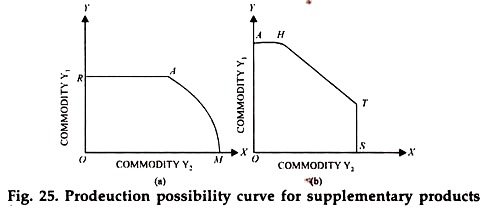
Two products are supplementary when the diversion of a given variable input from one product, say Y₂ to the other product, say Y₂ results in the increase in Y₂ without causing any decrease or increase in the production of Y₁ Fig. 25 (a) shows a production possibility curve for such supplementary products.

Fig. 25 (a) shows the two products to be supplementary upto point A because upto this point, the output of Y₂ can be increased without affecting the output of Y₁ After A, as in case of products which are initially complementary (Fig. 24), they become competitive to each other.

We must note here that supplementary relations between two products, in fact, show themselves up on both ends of the production possibility curve i.e., if Y₁ is supplementary Y₂ Y₂is supplementary to y₁ Fig. 25b).

We may like to search for an example of supplmentarity in production in agriculture. In crop production, much of the work is seasonal. There are periods when labour force is fully occupied and at other times, it is underemployed.

Sometimes in lean season such labour is used to produce products such as eggs, or pigs. These subsidiary products are obtained without any detrimental effect on the output of main products, of course, upto a certain limit.