Determination of Producer’s Equilibrium and Expansion Path

As we all know, producers generally strive hard to maximize profit at minimum cost.

A producer can attain equilibrium by applying the least cost combination of factors of production to attain maximum profit.

Therefore, he/she needs to decide the appropriate combination among different combinations of factors of production to get maximum profit at least cost.

The producers try to use ratios of factors in such a way so that maximum output can be obtained, while keeping the cost as low as possible. The decision of a producer depends on the principal of substitution. Suppose a producer has two factors of production, A and B. In these factors A can produce more output than B with the same amount of money spent on them.

This would make the producer to substitute A for B The producer equilibrium would be attained when the output produced by spending an additional unit of money (marginal rupee) on A is equal to the output produced by spending an additional unit of money on B. The producer would keep on substituting one input with the other to get maximum output till the producer equilibrium is not reached.

The marginal rupee spent on A would be represented as:

Marginal rupee spent on A= marginal product of A/price per unit

Suppose, the marginal output produced by A is 120 at Rs. 10 per unit, then

Marginal rupee spent on A = 120/10

= 12

Therefore, 12 is the additional output obtained by spending marginal rupee on A.

The producer equilibrium can be represented as follows:

MPa/Pa = MPb/Pb = …….. = MPn/Pn

In case the value of MPa/Pa is greater than MPb, then producers would substitute A for B.

Determination of Producer’s Equilibrium:

Producer’s equilibrium can be obtained with the help of isoquant and iso-cost line. An isoquant enables a producer to get those combinations of factor that yield maximum output.

On the other hand, iso-cost line provides the ratio of prices of factors of production and the amount that a producer is willing to spend. For attaining equilibrium, a producer needs to obtain a combination that helps in producing maximum output with the least price.

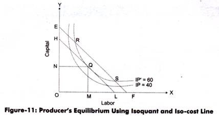
Figure- 11 shows the equilibrium position obtained with the help of isoquant and iso-cost line:

As shown in Figure-11, the producer can produce 60 units of output by using any combinations that is R, Q, and S, on curve IP’. He/she would select the combination that would obtain the lowest cost. It can be seen from Figure-11 that Q lies on the lowest iso- cost line and would yield same profit as on R and S points, at the lowest cost. In such a case, Q is the point of equilibrium; therefore, it would be selected by the producer.

Expansion Path:

In case, after attaining equilibrium, if a producer is willing to increase its production, then he/she needs to determine the combination that is required to reach a new equilibrium state. Let us consider Figure-11 in which the producer is willing to produce 60 units of output. Now, the producer wants to produce 80 units of output instead of 60 units.

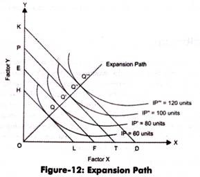
In such a case, the equilibrium would be achieved at the point Q’, which is shown in Figure-12:

In Figure-12, Q,’ would be the equilibrium point for producing 80 units of output. This is because at point Q,’ iso-cost line is tangent to isoquant curve of IP’. Similarly, the equilibrium point for producing 100 and 120 units are Q.” and Q,'”, respectively. When the points Q, Q’, Q”, and Q.'” are joined, a straight line is obtained, which is called expansion path or scale line.

This line is termed as scale line because producer needs to adjust its scale of production according to this line to achieve the output he/she desires. On the other hand, this line is also termed as expansion path because the producer needs to expand his/her output by following this path when the prices of factors remain constant. Producers would prefer to move along the scale line to increase the output to get maximum output at least cost with fixed factor prices.