Long-Run Production Function (With Diagram)

Production in the short run in which the functional relationship between input and output is explained assuming labor to be the only variable input, keeping capital constant.

In the long run production function, the relationship between input and output is explained under the condition when both, labor and capital, are variable inputs.

In the long run, the supply of both the inputs, labor and capital, is assumed to be elastic (changes frequently). Therefore, organizations can hire larger quantities of both the inputs. If larger quantities of both the inputs are employed, the level of production increases. In the long run, the functional relationship between changing scale of inputs and output is explained under laws of returns to scale. The laws of returns to scale can be explained with the help of isoquant technique.

Isoquant Curve:

The relationships between changing input and output is studied in the laws of returns to scale, which is based on production function and isoquant curve. The term isoquant has been derived from a Greek work iso, which means equal. Isoquant curve is the locus of points showing different combinations of capital and labor, which can be employed to produce same output.

It is also known as equal product curve or production indifference curve. Isoquant curve is almost similar to indifference curve. However, there are two dissimilarities between isoquant curve and indifference curve. Firstly, in the graphical representation, indifference curve takes into account two consumer goods, while isoquant curve uses two producer goods. Secondly, indifference curve measures the level of satisfaction, while isoquant curve measures output.

Some of the popular definitions of isoquant curve are as follows:

According to Ferguson, “An isoquant is a curve showing all possible combinations of inputs physically capable of producing a given level of output.”

According to Peterson, “An isoquant curve may be defined as a curve showing the possible combinations of two variable factors that can be used to produce the same total product”

From the aforementioned definitions, it can be concluded that the isoquant curve is generated by plotting different combinations of inputs on a graph. An isoquant curve provides the best combination of inputs at which the output is maximum.

Following are the assumptions of isoquant curve:

i. Assumes that there are only two inputs, labor and capital, to produce a product

ii. Assumes that capital, labor, and good are divisible in nature

iii. Assumes that capital and labor are able to substitute each other at diminishing rates because they are not perfect substitutes

iv. Assumes that technology of production is known

On the basis of these assumptions, isoquant curve can be drawn with the help of different combinations of capital and labor. The combinations are made such that it does not affect the output.

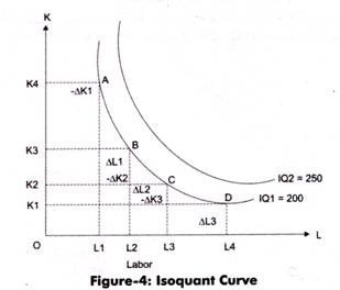
Figure-4 represents an isoquant curve for four combinations of capital and labor:

In Figure-4, IQ1 is the output for four combinations of capital and labor. Figure-4 shows that all along the curve for IQ1 the quantity of output is same that is 200 with the changing combinations of capital and labor. The four combinations on the IQ1 curve are represented by points A, B, C, and D.

Table-4 shows the relationship between input and output for IQ1 curve:

In Table-4, as we move from A to D, capital starts decreasing with the increase in labour. This shows that capital is substituted by labor, while keeping the output unaffected.

As discussed earlier, isoquant curve is almost similar to indifference curve. The properties of isoquant curve can be explained in terms of input and output.

Some of the properties of the isoquant curve are as follows:

i. Negative Slope:

Implies that the slope of isoquant curve is negative. This is because when capital (K) is increased, the quantity of labor (L) is reduced or vice versa, to keep the same level of output. As shown in Table-4, when the quantity of labor is increased from one unit to two units, the quantity of capital is decreased from four to three, to keep the level of output constant, which is 200.

ii. Convex to Origin:

Shows the substitution of inputs and diminishing marginal rate of technical substitution (which is discussed later) in economic region. This implies that marginal significance of one input (capital) in terms of another input (labor) diminishes along with the isoquant curve. For example, in Table-4, it can be seen when more and more units of capital are used to produce 200 units of output, less or less units of labor are used.

iii. Non-intersecting and Non-tangential:

Implies that two isoquant curves (as shown in Figure-4) cannot cut each other.

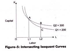
Figure-5 shows the intersection of two isoquant curves:

In Figure-5, the two isoquant curves intersect at point A. The point B on isoquant having Q2 = 300 and point C on isoquant curve having Q1 = 200 with the same amount of labor that is OL2. However, the capital is different that is BL2 in case of point B and CL2 in case of point C. A is the common point of isoquant for B and C points.

Now, according to isoquant definition, the output produced at A is the same as produced on B and C points. On isoquant curve Q1, the output produced at A and C is 200 while on Q2 curve the output priced at A and B is 300.

To make the input at point B and C equal, the following formula is used:

OL2 + BL2 = OL2 + CL2

BL2 = CL2

However according to Figure-5, BL2 > CL2 but the intersection of two isoquants implies that BL2 and CL2 are equal with respect to their output, which is not possible. Therefore, it is stated that isoquant curves cannot intersect; otherwise the law of production would not be applicable.

iv. Upper isoquant have high output:

Implies that upper curve of the isoquant curve produces more output than the curve beneath. This is because of the larger combination of input result in a larger output as compared to the curve that s beneath it. For example, in Figure-5 the value of capital at point B is greater than the capital at point C. Therefore, the output of curve Q2 is greater than the output of Q1.

Marginal Rate of Technical Substitution:

Marginal Rate of Technical Substitution (MRTS) is the quantity of one input (capital) that is reduced to increase the quantity of the other input (L), so that the output remains constant.

Table-5 shows the marginal rate of technical substitution:

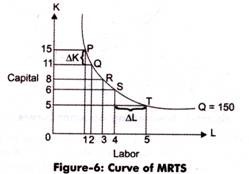
Table-5 shows that how much labor is required to replace one unit of capital while keeping the output same for all combinations of capital and labor, which is 150.

In such a case, MRTS can be calculated with the help of the following formula:

MRTS = ∆K/∆L

Where, ∆K = Change in Capital

∆L= Change in Labor

For example, in Table-5 at point Q MRTS can be calculated as follows:

∆K = new capital – old capital

∆K= 15 – 11

∆K = 4

∆L = 2 – 1

∆L= 1

Therefore, MRTS at point Q would be:

MRTS = ∆K/∆L

MRTS = 4/1 or 4:1

Similarly, we can calculate MRTS at different points, which are R, S, and T.

Figure-6 shows the curve of MRTS:

Forms of Isoquants:

The shape of an isoquant depends on the degree to which one input can be substituted by the other. Convex isoquant represents that there is a continuous substitution of one input variable by the other input variable at a diminishing rate.

However, in economics, there are other forms of isoquants, which are as follows:

i. Linear Isoquant:

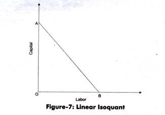
Refers to a straight line isoquant. Linear isoquant represents a perfect substitutability between the inputs, capital and labor, of the production function. It implies that a product can be produced by using either capital or labor or using both, if capital and labor are perfect substitutes of each other. Therefore, in a linear isoquant, MRTS between inputs remains constant.

The algebraic form of production function in case of linear isoquant is as follows:

Q = aK + BL

Here, Q is the weighted sum of K and L.

Slope of curve can be calculated with the help of following formula:

MP_K = ∆Q/∆K = a

MP_L = ∆Q/∆L = b

MRTS = MP_L/MP_K

MRTS = -b/a

However, linear isoquant does not have existence in the real world.

Figure-7 shows a linear isoquant:

ii. L-shaped Isoquant:

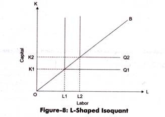
Refers to an isoquant in which the combination between capital and labor are in a fixed proportion. The graphical representation of fixed factor proportion isoquant is L in shape. The L-shaped isoquant represents that there is no substitution between labor and capital and they are assumed to be complementary goods.

It represents that only one combination of labor and capital is possible to produce a product with affixed proportion of inputs. For increasing the production, an organization needs to increase both inputs proportionately.

Figure-8 shows an L-shaped isoquant:

In Figure-8, it can be seen OK1 units of capital and OL1 units of labor are required for the production of Q1. On the other hand, to increase the production from Q1 to Q2, an organization needs to increase inputs from K1 to K2 and L1 to L2 both.

This relationship between capital and labor can be expressed as follows:

Q = f (K, L) = min (aK, bL)

Where, min = Q equals to lower of the two terms, aK and bL

For example, in case aK > bL, then Q = bL and in case aK < bL then, Q = aK.

L-shaped isoquant is applied in many production activities and techniques where labor and capital is in fixed proportion. For example, in the process of driving a car, only one machine and one labor is required, which is a fixed combination.

iii. Kinked Isoquant:

Refers to an isoquant that represents different combinations of labor and capital. These combinations can be used in different processes of production, but in fixed proportion. According to L-shaped isoquant, there would be only one combination between capital and labor in a fixed proportion. However, in real life, there can be several ways to perform production with different combinations of capital and labor.

For example, there are two machines in which one is large in size and can perform all the processes involved in production, while the other machine is small in size and can perform only one function of production process. In both the machines, combination of capital employed and labor used is different.

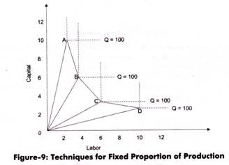
Let us understand kinked isoquant with the help of another example. For example, to produce 100 units of product X, an organization has used four different techniques of production with fixed-factor proportion.

The combination between inputs and their ratio is provided in Table-6:

In Table-6, OA, OB, OC, and OD represents the four production techniques. The fixed capital-labor ratio for OA technique is 10:2, for OB it is 6:3, for OC 4:6, and for OD is 3:10. Therefore, different production techniques use different fixed combinations of capital and labor.

The graphical representation of kinked isoquant is shown in Figure-9:

Elasticity of Factor Substitution:

We have studied that MRTS is associated with the slope of an isoquant and represents ratio of marginal changes in inputs. MRTS does not represent the substitutability between the two inputs, capital and labor, with different combinations of inputs.

However, it is important to measure the degree of substitutability between the two inputs. Therefore, economists have developed a formula for estimating the extent of substitutability between the two inputs, capital and labor, which is known as elasticity of factor substitution.

Elasticity of factor substitution (a) refers to the ratio of percentage change in capital-labor ratio to the percentage change in MRTS.

It is mathematically represented as follows:

σ = percentage change in capital labor ratio/percentage change in MRTS

Or,

σ = [(AK/AL) /AMRTS] * [MRTS/ (K/L)]

If change produced in capital-labor ratio by change in MRTS-is equal and in opposite direction, then σ = 1. If the change produced in capital-labor ratio is greater than the change in MRTS, then σ > 1. In case the change in capital-labor ratio is greater than the change in MRTS, then σ < 1. High elasticity of substitution between factors implies that the factors can easily substituted to each other, while a low elasticity represents that substitution of factors is possible to a certain extent.

The degree of elasticity depends on the shape of isoquant curve. If the shape of isoquant curve is linear and factors are perfect substitutes, then the substitution elasticity would be infinite. In case the factors are complementary to each other and isoquants are L-shaped, then the substitution elasticity is zero. The elasticity of substitution is negative between factors due to the inverse relation of factor-ratio and MRTS. The elasticity of substitution would be less as the convexity of the isoquant curve increases.