Profit-Maximising Behaviour of a Firm (With Diagram)

The following points highlight the top two approaches to explain the profit maximising behaviour of a firm.

Approach # 1. Equilibrium of a Firm—The Total Revenue and Total Cost Approach:

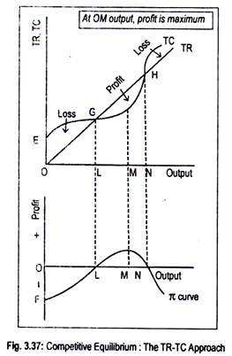
Profit becomes maximum irrespective of the market situation, when the difference between total revenue (TR) and total cost (TC) becomes the greatest. In Fig. 3.37, a TR curve for a perfectly competitive firm has been drawn. The TR curve starts from the origin and it rises in proportion to the rise in the volume of sales.

The TC curve starts from point E which lies above the origin. This means that costs are positive even if no output is produced. Such costs are called fixed costs of a firm. All these curves have been drawn in the upper panel of the figure. The bottom part of the figure shows various amounts of profit enjoyed by a firm at various volumes of output.

Below the level of output OL, the firm incurs a loss since TC exceeds TR. Only at the OL output level, TR equals TC and the firm earns only normal profit. Thus, point G is called break-even point. Now, if more than OL but less than ON output is produced, TR will exceed total cost and the firm will earn supernormal profit.

However, at the output level OM, as the difference between TR and TC is the greatest, profit is maximum. This is clear from the bottom panel of the figure where n is the profit curve. Below OL output level, profit curve lies below the origin indicating negative profit. Profit becomes zero at OL output level.

It becomes maximum at OM output level and, again, it reduces to zero (i.e., break-even point) when ON amount of output is produced. Beyond ON (or at ON), as TC exceeds TR, the firm incurs a loss. Now the profit curve has again entered the negative quadrant. Anyway, maximum profit is obtained at the output level OM, where the vertical distance between TR and TC curves is the maximum.

However, this approach is not free from defects. Firstly, a visual inspection suggests the maximum distance between TR and TC. But it is not easy to determine the exact volume of output where the vertical distance between TR and TC curves is the greatest.

Secondly, we do not know the price per unit of output sold. To obtain price, we will have to divide total revenue by the total output. In view of these problems associated with this approach, we use the marginalistic approach.

Approach # 2. Equilibrium of a Firm—the Marginal Revenue and Marginal Cost Approach:

Irrespective of the market conditions, a firm will stop production if total revenue falls short of total variable cost. Profit will be maximized at that point where MR and MC are equal to each other. For any output MR > MC, the firm will expand output.

Doing so, it will add more to its revenues them to its costs, thereby increasing profit. On the other hand, for the output MR > MC means that there is no incentive on the part of the firm to raise its output. If it decides to increase output when MC > MR, it will add more to its costs than to its revenues, thus reducing profit. Hence the profit-maximizing output occurs at that point when MR = MC.

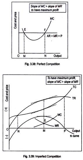
In Figs. 3.38 and 3.39, we have shown equilibrium of a firm under perfect and imperfect competition, respectively. Under perfect competition, AR = MR = P. It has been drawn parallel to the horizontal axis. MC curve is U-shaped. Profit is maximized when MR and MC are equal.

In Fig. 3.39, MC = MR at points E and F. Thus these are the two points where profit is maximized. One of the important properties of equilibrium is uniqueness. In other words, there cannot be more than one equilibrium point.

At point E, though MR = MC, it does not correspond to profit-maximizing situation.

If the firm expands output beyond OM, it will add more revenue than to its costs, since MR > MC. It will enjoy more profit by producing more output. Only at output ON will profit be maximized when MR = MC. Production beyond ON will entail a loss since MC > MR. So, a profit-maximizing firm always changes output toward the level at which MR = MC.

On the basis of the above discussion, one can conclude that there are two conditions for profit-maximization:

i. MC = MR, known as necessary condition or first-order condition (FOC); and

ii. MC curve must cut MR curve from below.

This condition may be modified in the following way:

Slope of MC must be greater than the slope of MR or the rate of change of MC must be greater than the rate of change of MR. This condition is called sufficient condition or second-order condition (SOC).

Note that, since MR is a horizontal curve, its slope is zero. At point E, slope of MC > slope of MR. This means that at point E, only FOC is satisfied, and not SOC. Equilibrium requires the fulfilment of both FOC and SOC, simultaneously. This occurs at point F. Corresponding to point F, ON is the profit-maximizing level of output.

In Fig 3.39, the imperfectly competitive firm is in equilibrium at point E where both FOC and SOC are satisfied. At OM output, profit is actually maximized since the difference between TR and T’C is the greatest π curve or the profit curve shows that profit is maximum at OM output.

Note that the gradients of the TR and TC curves (i.e., MR and MC, respectively) have identical slopes at OM output.

So total profit becomes maximum when the following two conditions (FOC and SOC) for equilibrium hold:

(i) MC= MR and

(ii) Slope of MC > slope of MR.

However, profit is zero both at ON and OP levels of output since, at these output levels, TR equals TC.