Relation between Total Revenue, Average Revenue and Marginal Revenue!
1. Both AR and MR are Calculated from TR:
The average cost and marginal costs are calculated from total cost. In the same fashion, average revenue and marginal revenue can also be calculated from total revenue.
2. When AR and MR are Parallel to X-axis:
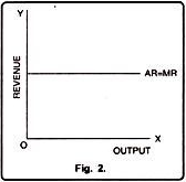
If average revenue and marginal revenue are parallel to horizontal axis then it means both AR and MR are equal to each other i.e. AR = MR. It has been shown with the help of table 2 and diagram 2.
From this table, it is clear that when output increases prices or AR remains the same i.e. Rs. 10.
ADVERTISEMENTS:
In figure 2, on X-axis, we have measured output and on Y-axis revenue. Average and marginal revenue are horizontal lines which are parallel to X-axis. It is a case under perfect competition.
3. When both AR and MR are Straight Lines:
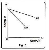
Under imperfect competition, when AR falls, MR also falls and it is always below AR line because there are large numbers of buyers and sellers, products are not homogeneous and the firms can enter or exit the market. It can be shown with the help of a table 3.
It is clear from the table that as price falls (AR falls) from Rs. 10 to Rs. 6, the total revenue (TR) increases from Rs. 10 to Rs. 30 at a diminishing rate. MR also falls from Rs. 10 to Rs. 2, MR is the rate at which the TR changes. It can also be drawn with the help of a Fig. 3.
In Fig. 3, AR and MR curves have been shown. It shows when AR curve falls MR curve also falls, and the MR curve will be below the AR curve. But, this situation exists only under monopoly and imperfect competition.
4. If AR Curve is Rising Upward from Left to Right:
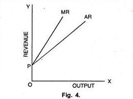
In case AR curve is rising upward from left to right, then MR curve will also move upward. It means MR will be greater than AR. This is shown with the help of a table 4 and Fig.4.
Table 4 shows that as AR or price increases from Rs. 10 to Rs. 14, units sold also go up from 1 to 5. In the same way, TR increases from Rs. 10 to Rs. 70 at an increasing rate. As a result, MR also increases from Rs. 10 to Rs. 18. In Fig. 4 we see that AR and MR both start from the same point as AR rises upwards from left to right. MR also follows the same trend i.e. above AR curve.
5. When AR and MR are Convex:
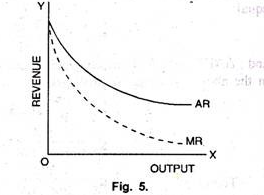
In fig. 5, AR and MR curves are convex to the origin. It means as more and more units of a commodity are sold, average revenue falls at lower speed. MR curve also moves in the same direction. The convexity shows that MR falls but at a faster speed.
6. When AR and MR are Concave:
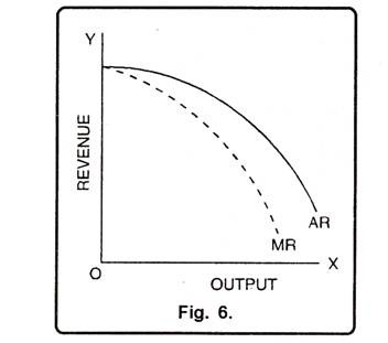
The figure 6 shows that if AR is concave to the origin, MR will also be concave to the origin. It means average revenue is falling at a higher rate for each additional unit of a commodity sold. Similar would be the case for MR curve.
7. Revenue and Elasticity:
The elasticity of demand, average revenue and marginal revenue has a close relationship. If a firm knows any two of the three elements viz; average revenue and marginal revenue then it can easily find out the third element i.e. elasticity of demand.
The formula for the calculation is:
ADVERTISEMENTS:
E = A / A-M
Where E = elasticity of demand; A = average revenue; M = marginal revenue
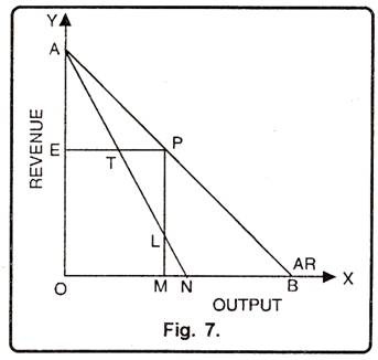
This method can be explained with the help of a Fig. 7.
ADVERTISEMENTS:
In this Fig. 7, revenue has been shown on OY-axis while quantity of goods on OX-axis. AB is the average revenue or demand curve and AN is the marginal revenue curve. At point P on demand curve, elasticity of demand is calculated with the formula,
Ep = Lower Portion / Upper Portion
We see in the figure that AAEP and APMB are similar, thus ratio of their sides is also equal.
Ep = PB/PA = PM/AE
ADVERTISEMENTS:
And; ∆AET and ∆PTL are congruent triangles, therefore PL=AE. Putting PL in place of AE in the above equation, we shall get
In this way, if value of Ep is one, it means that price elasticity of demand is unity. Similarly, if it is more than one, price elasticity of demand is greater than unity and if it is less than one, price elasticity of demand is less than unity.

