Solow’s Model of Growth (With Diagram)

The below mentioned article provides an overview on the Solow’s model of growth.

Introduction:

Prof. Robert M. Solow made his model an alternative to Harrod-Domar model of growth.

It ensures steady growth in the long run period without any pitfalls. Prof. Solow assumed that Harrod-Domar’s model was based on some unrealistic assumptions like fixed factor proportions, constant capital output ratio etc.

Solow has dropped these assumptions while formulating its model of long-run growth. Prof. Solow shows that by the introduction of the factors influencing economic growth, Harrod-Domar’s Model can be rationalised and instability can be reduced to some extent.

He has shown that if technical coefficients of production are assumed to be variable, the capital labour ratio may adjust itself to equilibrium ratio in course of time.

In Harrod-Domar’s model of steady growth, the economic system attains a knife-edge balance of equilibrium in growth in the long-run period.

This balance is established as a result of pulls and counter pulls exerted by natural growth rate (Gn) (which depends on the increase in labour force in the absence of technical changes) and warranted growth rate (Gw) (which depends on the saving and investment habits of household and firms).

However, the key parameter of Solow’s model is the substitutability between capital and labour. Prof. Solow demonstrates in his model that, “this fundamental opposition of warranted and natural rates turns out in the end to flow from the crucial assumption that production takes place under conditions of fixed proportions.”

The knife edge balance established under Harrodian steady growth path can be destroyed by a slight change in key parameters.

Prof. Solow retains the assumptions of constant rate of reproduction and constant saving ratio etc. and shows that substitutability between capital and labour can bring equality between warranted growth rate (Gw) and natural growth rate (Gn) and economy moves on the equilibrium path of growth.

In other words, according to Prof. Solow, the delicate balance between Gw and Gn depends upon the crucial assumption of fixed proportions in production. The knife edge equilibrium between Gw and Gn will disappear if this assumption is removed. Solow has provided solution to twin problems of disequilibrium between Gw and Gn and the instability of capitalist system.

In short, Prof. Solow has tried to build a model of economic growth by removing the basic assumptions of fixed proportions of the Harrod-Domar model. By removing this assumption, according to Prof. Solow, Harrodian path of steady growth can be freed from instability. In this way, this model admits the possibility of factor substitution.

Assumptions:

Solow’s model of long run growth is based on the following assumptions:

1. The production takes place according to the linear homogeneous production function of first degree of the form

Y = F (K, L)

Y = Output

K = Capital Stock

L = Supply of labour force

The above function is neo-classic in nature. There is constant returns to scale based on capital and labour substitutability and diminishing marginal productivities. The constant returns to scale means if all inputs are changed proportionately, the output will also change proportionately. The production function can be given as aY = F (aK, al)

2. The relationship between the behaviour of savings and investment in relation to changes in output. It implies that saving is the constant fraction of the level of output. In this way, Solow adopts the Harrodian assumption that investment is in direct and rigid proportion to income.

In symbolic terms, it can be expressed as follows:

I = dk/ dt = sY

Where

S—Propensity to save.

K—Capital Stock, so that investment I is equal

3. The growth rate of labour force is exogenously determined. It grows at an exponential rate given by

L = L₀ e^nt

Where L—’Total available supply of labour.

n—Constant relative rate at which labour force grows.

4. There is full employment in the economy.

5. The two factors of production are capital and labour and they are paid according to their physical productivities.

6. Labour and capital are substitutable for each other.

7. Investment is not of depreciation and replacement charges.

8. Technical progress does not influence the productivity and efficiency of labour.

9. There is flexible system of price-wage interest.

10. Available capital stock is fully utilized.

Following these above assumptions, Prof. Solow tries to show that with variable technical co-efficient, capital labour ratio will tend to adjust itself through time towards the direction of equilibrium ratio. If the initial ratio of capital labour ratio is more, capital and output will grow more slowly than labour force and vice-versa.

To achieve sustained growth, it is necessary that the investment should increase at such a rate that capital and labour grow proportionately i.e. capital labour ratio is maintained.

Solow’s model of long-run growth can be explained in two ways:

A. Non-Mathematical Explanation.

B. Mathematical Explanation.

A. Non-Mathematical Explanation:

According to Prof. Solow, for attaining long run growth, let us assume that capital and labour both increase but capital increases at a faster rate than labour so that the capital labour ratio is high. As the capital labour ratio increases, the output per worker declines and as a result national income falls.

The savings of the community decline and in turn investment and capital also decrease. The process of decline continues till the growth of capital becomes equal to the growth rate of labour. Consequently, capital labour ratio and capital output ratio remain constant and this ratio is popularly known as “Equilibrium Ratio”.

Prof. Solow has assumed technical coefficients of production to be variable, so that the capital labour ratio may adjust itself to equilibrium ratio. If the capital labour ratio is larger than equilibrium ratio, than that of the growth of capital and output capital would be lesser than labour force. At some time, the two ratios would be equal to each other.

In other words, this is the steady growth, according to Prof. Solow as there is the steady growth there is a tendency to the equilibrium path. It must be noted here that the capital-labour ratio may be either higher or lower.

Like other economies, Prof. Solow also considers that the most important feature of an underdeveloped economy is dual economy. This economy consists of two sectors-capital sector or industrial sector and labour sector or agricultural sector. In industrial sector, the rate of accumulation of capital is more than rate of absorption of labour.

With the help of variable technical coefficients many employment opportunities can be created. In agricultural sector, real wages and productivity per worker is low. To achieve sustained growth, the capital labour ratio must be high and underdeveloped economies must follow Prof. Solow to attain the steady growth.

This model also exhibits the possibility of multiple equilibrium positions. The position of unstable equilibrium will arise when the rate of growth is not equal to the capital labour ratio. There are other two stable equilibrium points with high capital labour ratio and the other with low capital labour ratio.

If the growth process starts with high capital labour ratio, then the development variables will move in forward direction with faster speed and the entire system will grow with high rate of growth. On the other hand, if the growth process starts with low capital labour ratio then the development variables will move in forward direction with lesser speed.

To conclude the discussion, it is said that high capital labour ratio or capital intension is very beneficial for the development and growth of capitalist sector and on the contrary, low capital-labour ratio or labour-intensive technique is beneficial for the growth of labour sector.

B. Mathematical Explanation:

This model assumes the production of a single composite commodity in the economy. Its rate of production is Y (t) which represents the real income of the community. A part of the output is consumed and the rest is saved and invested somewhere.

The proportion of output saved is denoted by s. Therefore, the rate of saving would be sY (t). The capital stock of the community is denoted by K it). The rate of increase in capital stock is given by dk/dt and it gives net investment.

Since investment is equal to saving so we have following identity:

K = sY … (1)

Since output is produced by capital and labour, so the production function is given by

Y = F (K, L) … (2)

Putting the value of Y from (2) in (1) we get

S = s F (K, L) … (3)

Where

L is total employment

F is functional relationship

Equation (3) represents the supply side of the system. Now we are to include demand side too. As a result of exogenous population growth, the labour force is assumed to grow at a constant rate relative to n. Thus,

L (t) = L₀e^nt … (4)

Where

L—Available supply of labour

Putting the value of L in equation (3) we get

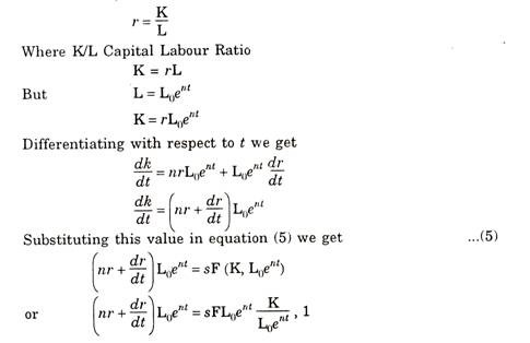
K = sF (K, L₀e^nt) …(5)

The right hand of the equation (4) shows the rate of growth of labour force from period o to t or it can be regarded as supply curve for labour.

“It says that the exponentially growing labour force is offered for employment completely in elastically. The labour supply curve is a vertical line, which shifts to the right in time as the labour force grows. Then the real wage rate adjusts so that all available labour is employed and the marginal productivity equation determines the wage rate which will actually rule.”

If the time path of capital stock and of labour force is known, the corresponding time path of real output can be computed from the production function. Thus, the time path of real wage rate is calculated by marginal productivity equation.

The process of growth has been explained by Prof. Solow as, “At any moment of time the available labour supply is given by (4) and available stock of capital is also a datum. Since the real return to factors will adjust to bring about full employment of labour and capital we can use the production function (2) to find the current rate of output. Then the propensity to save tells us how much net output will be saved and invested. Hence, we know the net accumulation of capital during the current period. Added to the already accumulated stock this gives us the capital available for the next period and the whole process can be repeated.”

Possible Growth Patterns:

To find out whether there is always a capital accumulation path consistent with any rate of growth of labour force, we should know the accurate shape of production function otherwise we cannot find the exact solution.

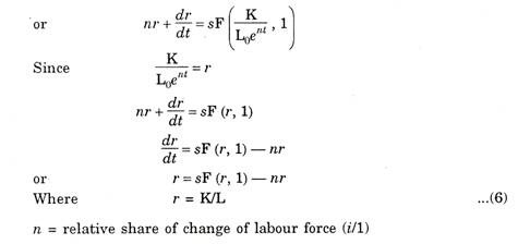
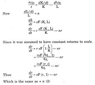
For this, Solow has introduced a new variable:

The function F(r, 1) gives output per worker or it is the total product curve as varying amounts ‘r’ of capital are employed with one unit of labour. The equation (6) states that, “the rate of change of the capital labour ratio as the difference of two terms, one representing the increment of capital and one the increment of labour.”

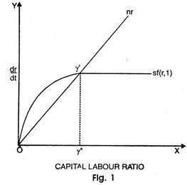
The diagrammatic representation of the above growth pattern is as under:

In diagram 1, the line passing through origin is nr. The total productivity curve is the function of SF (r, 1) and this curve is convex to upward. The implication is that to make the output positive it must be necessary that input must also be positive i.e. diminishing marginal productivity of capital. At the point, of intersection i.e. nr = sf (r, 1) and r’ = o when r’ = o then capital labour ratio corresponds to point r* is established.

Now capital and labour will grow proportionately. Since Prof. Solow considers constant returns to scale, real output will grow at the same rate of n and output per head of labour, force will remain constant.

In mathematical terms, it can be explained as:

Path of Divergence:

Here we are to discuss the behaviour of capital labour ratio, if there is divergence between r and r”. There are two cases:

(i) When r > r*

(ii) When r < r*

If r > r* then we are towards the right of intersection point. Now nr > sF (r, 1) and from equation (6) it is easily shown that r will decrease to r*. On the other hand if we move towards left of the intersection point where nr < sF (r, 1), r>o and r will increase towards r*. Thus, equilibrium will be established at point E and sustained growth will be achieved. Thus, the equilibrium value of r* is stable.

According to Prof. Solow, “Whatever the initial value of the capital labour ratio, the system will develop towards a state of balanced growth at a natural rate. If the initial capital stock is below the equilibrium ratio, capital and output will grow at a faster rate than the labour force until the equilibrium ratio is approached. If the initial ratio is above the equilibrium value, capital and output will grow more slowly than the labour force. The growth of output is always intermediate between those of labour and capital.”

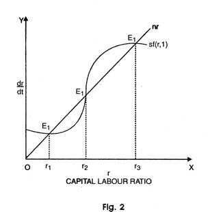
The stability depends upon the shape of the productivity curve sF(r, 1) and it is explained with the help of a diagram given below:

In the figure 2. the productivity curve sf (r, 1) intersects the ray nr at three different points E₁ , E₂ , E₃. The corresponding capital labour ratio is r₁, r₂ and r₃. The points are r₃ stable but r₂ is not stable. Taking point r₁ first if we move slightly towards right nr > sf(r, 1) and r is negative implying that r decreases.

Thus, it has a tendency to slip back to r₁ .If we move slightly towards its left nr < sf (r, 1) and r is positive which shows that r increases and there is a tendency to move upto point r₁. Therefore, a slight movement away from r₁ creates conditions that forces a movement towards showing that r₁ is a point of stable equilibrium.

Likewise, we can show that r₃ is also a point of stable equilibrium. If we move slightly towards right of r₂, sf (r, 1) nr and r is positive and there is a tendency to move away from r₂.

On the other hand, if we move slightly towards left of r₂ nr > sf (r, 1) so that r is negative and it has a tendency to slip downwards towards r₁. Therefore depending upon initial capital labour ratio, the system will develop to balanced growth at capital labour ratio r₁ and r₃. If the initial ratio is between o and r₂, the equilibrium is at r₁ and if the ratio is higher than r₂ then equilibrium is at r₃.

To conclude Solow puts, “When production takes place under neoclassical conditions of variable proportions and constant returns to scale, no simple opposition between natural and warranted rates of growth is possible. There may not be any knife edge. The system can adjust to any given rate of growth of labour force and eventually approach a state of steady proportional expansion” i.e.

∆K/K = ∆L/L = ∆Y/Y

 

Unlike Harrodian model, Solow’s model also does not apply to development’ problem of under-developed countries. Most of the under-developed countries are either in pre take-off or ‘take-off condition and this model does not analyse any policy formulation to meet the problems of under-developed countries.

But certain elements from the Solow model are still valid and can be used to chalk out the problem of under- development. The remarkable feature of Solow model is that it provides deep insight into the nature and type of expansion experienced by the two sectors of under-developed countries.

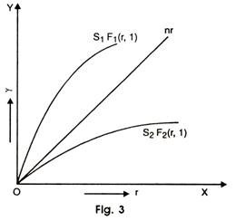
The interpretation of under- development is explained with the help of a diagram 3 given as next:

The line nr represents the balanced requirement line. When the warranted growth rate and natural growth rate are equal then steady growth is achieved.

Along this path, there is full employment and unchanging capital labour ratio. The curve represented by s₁ƒ₁ (r, 1) gives productive system in terms of both output and savings. On the other hand s₂ƒ₂ (r, 1) gives unproductive system and the per capita income and savings would decline. Both the systems have low marginal productivity.

The first system can be identified by industrial sector of under-developed countries which tends to grow with ever increasing intakes of capital in relation to labour. The second system conforms to the agrarian sector of under-developed countries. There is more labour supply due to rapid population growth. Investment is also positive.

The bottleneck of skilled labour holds back the expansion of industrial sector of under-developed countries.

The marginal productivity of labour is bound to fall and as it falls below the minimum real wage rates, disguised unemployment would rear its head. If the real wage rate is fixed at certain level, then employment is such that it can maintain marginal product of labour at this level.

Once the initial growth of population has occurred and land has become scarce, the real wage rate tends to be fixed at certain level, though the marginal productivity declines. The result of this is disguised unemployment.

In nut-shell, we can conclude the discussion of validity of Solow’s model is that there are certain elements which could be gainfully utilized for analysing the problem of under-development. The phenomenon of technological dualism which is commonly prevalent in these economies can be better explained in terms of Solow’s model.

Though, Solow’s model is basically embedded in a different setting, yet its concept of technical co-efficient provides elegant and simple theoretical apparatus to solve the problems of under-development.

Applicability to Underdeveloped Countries:

Unlike Harrodian model, Solow’s model also does not apply to development’ problem of under-developed countries. Most of the under-developed countries are either in pre take-off or ‘take-off condition and this model does not analyse any policy formulation to meet the problems of under-developed countries.

But certain elements from the Solow model are still valid and can be used to chalk out the problem of under- development. The remarkable feature of Solow model is that it provides deep insight into the nature and type of expansion experienced by the two sectors of under-developed countries.

The interpretation of under- development is explained with the help of a diagram 3 given as next:

The line nr represents the balanced requirement line. When the warranted growth rate and natural growth rate are equal then steady growth is achieved. Along this path, there is full employment and unchanging capital labour ratio.

The curve represented by s₁ƒ₁ (r, 1) gives productive system in terms of both output and savings. On the other hand s₂ƒ₂ (r, 1) gives unproductive system and the per capita income and savings would decline. Both the systems have low marginal productivity.

The first system can be identified by industrial sector of under-developed countries which tends to grow with ever increasing intakes of capital in relation to labour. The second system conforms to the agrarian sector of under-developed countries.

There is more labour supply due to rapid population growth. Investment is also positive. The bottleneck of skilled labour holds back the expansion of industrial sector of under-developed countries.

The marginal productivity of labour is bound to fall and as it falls below the minimum real wage rates, disguised unemployment would rear its head. If the real wage rate is fixed at certain level, then employment is such that it can maintain marginal product of labour at this level.

Once the initial growth of population has occurred and land has become scarce, the real wage rate tends to be fixed at certain level, though the marginal productivity declines. The result of this is disguised unemployment.

In nut-shell, we can conclude the discussion of validity of Solow’s model is that there are certain elements which could be gainfully utilized for analysing the problem of under-development. The phenomenon of technological dualism which is commonly prevalent in these economies can be better explained in terms of Solow’s model.

Though, Solow’s model is basically embedded in a different setting, yet its concept of technical co-efficient provides elegant and simple theoretical apparatus to solve the problems of under-development.

Merits of the Model:

Solow’s growth model is a unique and splendid contribution to economic growth theory. It establishes the stability of the steady-state growth through a very simple and elementary adjustment mechanism.

Certainly, the analysis is definitely an improvement over Harrod-Domar model, as he succeeded in demonstrating the stability of the balanced equilibrium growth by implying neo-classical ideas. In fact, Solow’ growth model marks a brake through in the history of economic growth.

The merits of Prof. Solow’s model are under-mentioned:

(i) Being a pioneer of neo-classical model, Solow retains the main features of Harrod-Domar model like homogeneous capital, a proportional saving function and a given growth rate in the labour forces.

(ii) By introducing the possibility of substitution between labour and capital, he gives the growth process and adjustability and gives more realistic touch.

(iii) He considers a continuous production function in analysing the process of growth.

(iv) Prof. Solow demonstrates the steady-state growth paths.

(v) He successfully shunted aside all the difficulties and rigidities of modern Keynesian income analysis.

(vi) The long-run rate of growth is determined by an expanding labour force and technical process.

Short Comings of the Model:

1. No Study of the Problem of Balance between G and Gw:

Solow takes up only the problem of balance between warranted growth (Gw) and natural growth (Gn) but it does not take into account the problem of balance between warranted growth and the actual growth (G and Gw).

2. Absence of Investment Function:

There is a absence of investment function in Solow’s model and once it is introduced, problem of instability will immediately reappear in the model as in the case of Harrodian model of growth.

3. Flexibility of Factor Price may bring Certain Problems:

Prof. Solow assumed the flexibility of factor prices but it may bring certain difficulties in the path of steady growth.

For example, the rate of interest may be prevented from falling below a certain minimum level and this may in turn, prevent the capital output ratio from rising to a level necessary for sustained growth.

4. Unrealistic Assumptions:

Solow’s model is based on the unrealistic assumption that capital is homogeneous and malleable. But capital goods are highly heterogeneous and may create the problem of aggregation. In short, it is not easy to arrive at the path of steady growth when there are varieties of capital goods in the market.

5. No Study of Technical Progress:

This model has left the study of technological progress. He has merely treated it as an exogenous factor in the growth process. He neglects the problem of inducing technical progress through the process of learning, investment and capital accumulation.

6. Ignores the Composition of Capital Stock:

Another defect of Prof. Solow’s model is that it totally ignores the problem of composition of capital stock and assumes capital as a homogeneous factor which is unrealistic in the dynamic world of today. Prof. Kaldor has forged a link between the two by making learning a function of investment.