Let us learn about the Derivation of the Market Supply Curve.
To get total or market supply, we have to add the supplies of all the producers of a product. Thus the market supply of a good is the sum of quantities of that good the individual firms are willing to offer for sale at a given time period. Suppose, there are two producers of X, viz. products A and B, in an area. Both of them supply at the same point of time.
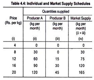
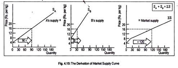
We show the supply schedule and the supply curve of the first and second firm producers i.e., A and B, in Table 4.4 and Fig. 4.15. Here we assume that the minimum price at which Firm B can offer a positive quantity (i.e., at Rs. 12) is higher than required by Firm A (i.e., Rs. 8).
The market supply is derived simply by adding the quantities supplied at each price by the two producers. Thus, we see that when the market price of X is Rs. 8, producer A offers a positive quantity (viz., 30 kg), but producer B offers nothing. So, market supply is the same as the individual supply (i.e., the amount offered by producer A).
Producer B is less efficient than producer A, i.e., B’s cost per unit is higher than that of A. So at this low price (Rs. 8 per kg), producer B is not willing to offer good X for sale in the market. However, as price rises to Rs. 12 per kg, producer A offers 60 kg and producer B 15 kg. Market supply is therefore 75 (= 60 + 15) kg. At each price the market supply is the sum of the quantities offered by A and B as the Table 4.4 indicates.
The market supply curve shown in Fig. 4.15 is arrived at by adding up the supply curves of the two producers (It would, however, be obtained straightway by plotting the information contained in columns (i) and (iv) in Table 4.4). SA is the supply curve of producer A and SB is that of B. Both these curves are upward rising.
ADVERTISEMENTS:
Thus, the market supply curve is the horizontal addition of the individual supply curves. Thus, when the market price is Rs. 16 per kg, the market supply is 120 kg, which is the sum of supplies of 90 kg and 30 kg of the two producers, respectively. If we repeat the same exercise for other prices we get a number of points.
The locus of all such points is the market supply curve S.
If we assume that there are 100 producers of X, and all are alike in all respects, then each of them would offer E.O.M.A.M.—10 the same quantity at all possible prices. In this case the market supply curve would be a 100-fold extension of the single firm’s supply curve. Like the supply curve of an individual firm, the market supply curve also slopes upward from left to the right.
To sum up, the supply of any commodity per given period of time at any given price depends on the cost incurred in producing it. It may be noted that both individual firms and the industry, as a whole, will be influenced by changes in prices.
ADVERTISEMENTS:
In the industry, if price increases, this will increase the level of profit. Consequently, new firms will enter the industry while existing firms will increase their own outputs. On the other hand, if price falls, we would expect firms to supply less of a commodity.
Once we understand this relationship between price and the quantity supplied, the first law of supply becomes reasonably obvious.
It states that:
More will tend to be supplied at a higher price than at a lower price—and this generalization is demonstrated by an upward sloping supply curve.

