Supply Curve of a Firm and Industry (With Diagram)

Supply Curve of a Firm and Industry: Short-Run and Long-Run Supply Curve!

Supply curve indicates the relationship between price and quantity supplied. In other words, supply curve shows the quantities that a seller is willing to sell at different prices.

According to Dorfman, “Supply curve is that curve which indicates various quantities supplied by the firm at different prices”. The concept of supply curve applies only under the conditions of perfect competition.

Supply curve can be divided into two parts as:

A. Short Run Supply Curve

B. Long Run Supply Curve

A. Short Run Supply Curve

(i) Short Run Supply Curve of a Firm:

Short run is a period in which supply can be changed by changing only the variable factors, fixed factors remaining the same. That way, if the firm shuts down, it has to bear fixed costs. That is why in the short run, the firm will supply commodity till price is either greater or equal to average variable cost. Thus a firm will continue supplying the commodity till marginal cost is equal to price or average revenue. Under perfect competition average revenue is equal to marginal revenue, so the firm will produce up to that point where marginal revenue and marginal cost are equal.

Short run supply curve of a perfectly competitive firm is that portion of marginal cost curve which is above average variable cost curve. According to C.E. Ferguson, “The short run supply curve of a firm in perfect competition is precisely its Marginal Cost Curve for all rates of output equal to or greater than the rate of output associated with minimum average variable cost.”

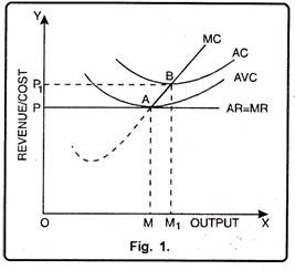
Prof. Bilas has defined it in simple words, “The Firm’s short period supply curve is that portion of its marginal cost curve that lies-above the minimum point of the average variable cost curve.” However, short run supply curve of a firm can be shown with the help of fig. 1.

From fig. 1 it is clear that there is no supply if price is below OP. At price less than OP, the firm will not be covering its average variable cost. At OP price, OM is the supply. In this case, firms’ marginal revenue and marginal cost cut each other at A, OM is equilibrium output. If price goes up to OP1, the firm will produce OM1 output. This firm’s short run supply curve starts from A upwards i.e., thick line AB.

(ii) Short Run Supply Curve of an Industry:

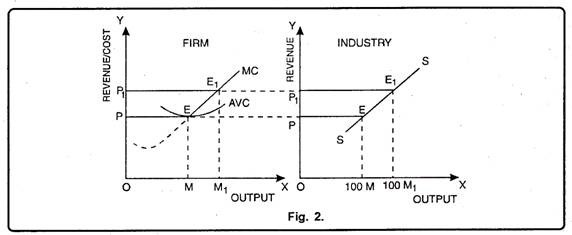
An industry is a blend of firms producing homogeneous goods. That way, supply curve of an industry is a lateral summation of all firms. This can be made clear with the help of a Fig. 2.

Here, we have assumed that different firms in the industry are producing identical products.

Each firm at OP price is producing OM output. It is because all firms have identical costs. At OP price, supply of industry is 100 x M = 100M.

Similarly at OP₁ price, all the firms of industry are producing 100 xM₁ =100M₁ quantity of output. These quantities will be called supply or output of industry. SS is the supply curve of industry. Point E shows that at OP price firm’s supply is OM and an industry’s total supply is 100 × M = 100M.

At OP₁ price, firm’s supply is OM1 and industry’s supply is 100M). We get industry’s supply curve by joining points E and E₁.

Thus, under perfect competition, lateral summation of that part of short run marginal cost curves of the firms which lie above the average variable cost constitutes the supply curve of the industry. According to Stonier and Hague, “short run supply curve of a competitive industry will always slope upwards since the short run marginal cost curve of the industrial firms always slope upward.”

B. Long Run Supply Curve:

Long run supply curve can also be analyzed from firm and industry’s point of view:

1. Long Run Supply Curve of a Firm:

Long run is a period in which supply can be changed by changing all the factors of production. There is no distinction between fixed and variable factors. In the long run, firm produces only at minimum average cost. In this situation, long run marginal cost, marginal revenue, average revenue and long run average cost are equal i.e., LMCMR (= AR)LAC (minimum). The firm is enjoying only normal profits.

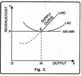
So that position of marginal cost curve will determine the supply curve which is above the minimum average variable cost. The point where minimum average cost is equal to marginal cost is called optimum production. Thus Long Run Supply Curve of a firm is that portion of its marginal cost curve that lies above the minimum point of the average cost curve.

In figure 3 the firm is in equilibrium at point E where MRLMC (=AR). AC is minimum corresponding to this point. This point E is also called optimum point because at this point MR=LMCAR minimum LAC. That portion of LMC which is above E is called long run supply curve.

2. Long Run Supply Curve of an Industry:

In the long run, industry’s supply curve is determined by the supply curve of firms in the long run. Long run supply curve in the long run is not lateral summation of the short run supply curves. Industry’s long run supply curve depends upon the change in the optimum size of firms and change in the number of firms.

It is on account of two reasons:

(i) In the long run, firms continue to enter into and exit from the industry,

(ii) Firms get economies and diseconomies of scale. This displaces the long run marginal cost (LMC).

Due to these reasons, long run supply curve of industry is not the lateral summation of supply curve of firms. In reality, long run supply curve of industry can be known from the long run optimum production of firms multiplied by the number of firms in an industry.

LRS_i, = Q x N

Where LRS₁ is long run supply curve of industry. Q is the optimum output of a firm and N, the number of firms.