Here is a term paper on the ‘Utility Function’ for class 9, 10, 11 and 12. Find paragraphs, long and short term papers on the ‘Utility Function’ especially written for school and college students.
Term Paper on Utility Function
Term Paper Contents:
- Term Paper on the Introduction to Utility Function
- Term Paper on the Lexicographic Ordering
- Term Paper on the Demand Function
- Term Paper on the Indirect Utility Function
- Term Paper on the Expenditure Function
- Term Paper on the Measures of Risk Aversion
Term Paper # 1. Introduction to the Utility Function:
ADVERTISEMENTS:
In microeconomics, consumer’s utility from consuming different commodities can be measured. Suppose the utility function u(x) assigns a numerical value to each element of x then the ranking of the elements of x is marked in accordance with the individual’s preference. Then, a function u: X → R is a utility function. It is representing preference relation » if for all x, y ϵ x , x ≥ y ↔ u(x) ≥ u(y) for any strict increasing function f: R → R and U(x) = f(u(x)) is a new utility function.
It is representing the same preferences as u (.). It is only the ranking that matter of alternative choices. After all, it is consumer’s preference and they are assigned some numbers. We can measure it with different examples. The ordinal utility function is known as the properties of the utility function. They are constant for any strictly increasing transformation preference relation and it is associated with a utility function. It is an ordinal property of utility function.
Property 1:
The consumer preference relation ≥ can be represented by a utility function only if it is rational.
ADVERTISEMENTS:
Solution:
Suppose a utility function that represents consumer preferences ≥ then ≥ must be complete and transitive.
It is explained with the help of properties as follows:
1. Complete:
ADVERTISEMENTS:
Suppose utility {u (.)} is a real valued function defined of x then it must be that for any x, y ϵ x either u(x) ≥ u(y) or u(y) ≥ u(x). But u(.) is a utility function and it is representing ≥, this implies that x ≥ y or that y ≥ x. Here, ≥ must be complete.
2. Transitivity:
Suppose x ≥ y and y ≥ z because u(.) represents ≥. We must have u(x) ≥ u(y) and u(y) ≥ u(z). Therefore, u(x) ≥ u(z). This is because u(.) represents ≥ and this implies x ≥ z. It is shown that x ≥ y and y ≥ z imply x ≥ z in this way transitivity is established. We have already explained it in above paragraph. Above two properties are also explained with the consumer choice rule.
Choice Rule of Consumer:
The preferences for commodities are nothing but the choices made by the consumer. Consumer has number of choices in his/her routine life. Choices for particular commodities are perfect and they are done after some mental exercise or psychology. While choosing preferences, consumer is ready to choose different products depending on their habits and likeness. In other words, the preference is a choice or it is a decision made by consumer. Consumer often faces a tradeoff between purchasing small quantities of a high quality and expensive products and large quantities of a lower quality and hence cheaper product.
In the simplest model, a sequence of people, each in turn choose one of two options, A or B, with each person observing all of his/her predecessors choice. They have common preferences over the two choices but do not know which is better. Rather, they receive independent and equally strong private binary signals about the right choice. In this setting, rational agents herd. Once the pattern of signals leads to two more choices of one action than the other, all subsequent people ignore their signals and take that same action.
The choice behavior is a choice structure sets and each set has two types. Firstly, S is a family of nonempty subsets of x. Every element of s is a set $ϵx. The element $ϵs is budget sets. The s set is a list of all choices available to consumer. It includes all subset of x. Secondly, the c is a choice rule that assigns a nonempty set of chosen elements c(h,i). For each budget set, it is written as $ϵs. When c ($) contains a single elements of c ($) then it is the alternatives in $. The consumer might choose such alternatives. They are his/her acceptable alternatives. Consumer repeatedly faces the problem of choosing an alternative from set $.
Term Paper # 2. Lexicographic Ordering:
The lexicographic ordering is known as lexical order. It is mathematical concept and it supports the assumption of continuity. It works with a numerical representation of consumers preference ordering. Sometimes, the numbers are not true because they are individual specific ordering and they get change from time to time. Lexicographic ordering assumes the simple utility maximization and function. It satisfies the four assumptions of lexicographic ordering ⎯ the continuity, transitivity, reflexivity and non-satiation. Such assumptions are important to build the demand function.
ADVERTISEMENTS:
Such demand function do not required the continuity assumption. If any consumer orders two commodities and both commodities are necessary for him then he/she consumes the commodities in particular proportion. The two commodities are ordered in the different fashion or form. Consumption of both commodities will add to a utility function.
It can be shown to satisfy first four assumptions that are:
1. Completeness,
2. Transitivity,
ADVERTISEMENTS:
3. Reflexivity and
4. Non-satiation.
It can be shown to give rise to well defined demand function, which implies that the continuity assumption is not necessary for their existence.
Theorem:
ADVERTISEMENTS:
Suppose we assume that there are two goods and they are ordered by the consumer because he/she likes those commodities.
The ordering can take place m the following form:
In the model, consumer prefers a bundle with more of first goods in consumption basket. Consumer is regardless of the second goods quantity. Sometimes, the consumer’s bundle contains the same quantity of first and second good. But the quantity of the second commodity matters for the consumer. But the presence for the two commodities is depending on the consumer’s habit of consumption and preferences. We can take an example of a drunkard man.
ADVERTISEMENTS:
He requires wine and bread in consumption basket. He prefers more wine in his bundle but at the same time, bread is also important for him. It is his choice to have the different combinations of wine and bread. A drunkard man would prefer more wine and less bread in his consumption bundle. Sometimes he will ensure the same amount of bread and wine. It is called as the Lexicographic ordering.
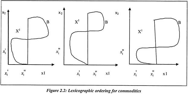
If we consider a consumption bundle x'(x’1, x”2) with wine and bread then all the points in B are preferred to wine. The other quantity is preferred of bread. There are three figures presented with different combinations of bread and wine. First figure shows the equal proportion of wine and bread in consumption basket. Second diagram shows less wine and the more bread is preferred. Third diagram shows that more wine and less bread is preferred. It is an individual preference and it is difficult to measure such choices. They are the preferences of drunkard man or woman. Such ordering is difficult to study all the time.
Criticism:
Suppose the drunker chooses wine arbitrarily, then the other points in the shape are for bread only but the lexicographic ordering is criticized. Firstly, it does not satisfy the continuity assumption. For continuity assumption, the points should have continuous curve. But the figure 2.2 shows the indifference set which are the assumed points and it is not a continuous curve. Indifference curve assumes that the two commodities are indifferent.
Suppose, we reduce the small amount of wine in the bundle to replace the bread then we find that no amount of bread can be replaced for wine. Therefore there is no continuity in the lexicographic ordering. It is known to all that drunker men/women prefer more wine than bread. Secondly, it is not possible to represent the use of utility function through lexicographic ordering.
ADVERTISEMENTS:
If we divide the real line into non-empty disjoint bounded intervals, the set of these intervals are not countable. The positive half of the real line is a countable and it must be false. It is difficult to collect data of lexicographic ordering. Similarly inter and intra individual choices get differ all the times.
Term Paper # 3. Demand Function:
From the lexicographic ordering, we can assume that the drunkard man/woman has M income. Suppose he/she is facing a price p1 for one bottle for wine and price p2per bread then she/he is free to spend his/her entire income on wine.
Therefore the demand function can be written as:
Here, X2 = 0 because drunkard does not spend his income on bread. The demand for the drunkard man/woman is just a rectangular hyperbola (x1, p1). The demand function for bread (x2, p2) is a space in the vertical axis.
ADVERTISEMENTS:
Existence of Utility Function:
The lexicographic ordering satisfies the completeness, reflexivity, transitivity, and new satiation. But lexicographic ordering does not satisfy the demand of goods. It only gives the preference of two commodities. The continuity assumption guarantees that a continuous increasing utility function can be found to represent the preference ordering.
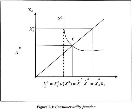
The figure 2.3 shows that the indifference curve is a continuous. There are two commodities x2 and x1 which are shown on x and y axis. The equilibrium point E is intersecting at 45° line. Any point on the indifference curve (x0) is associated with real number u(x0). In the diagram, E is a point at which the indifference curve x0 cuts the 45° line. The utility (u) values on the axis are a utility function for consumer. The indifference bundles have the same utility values but the higher preferred bundles have higher utility values.
In the figure 2.3, there exists utility function that is u (x’). In a given bundle x0 = (x01……. .x0n), the consumer chooses the X0 and X̅0. We have assumed that two commodities are indifferent. It means X̅0 = X0. Such assumption satisfies the continuity, transitivity etc. We also assumed that u(x0) = X̅0 equal to u(X0) = X̅0.
Such points are shown as follows:
The transitivity and non-satiation assumption shows that x values for 1 .x > x0 strictly greater than the complementary sub interval for which x0 > 1 .x. The formal rule interval has a lower bound at lower level. The latter rule interval has a least upper bound. These bounds must be same.
ADVERTISEMENTS:
Utility Theorem:
The u(x) constructed for two bundles x0, x1 satisfy the definition of a utility function.
Above function can be proved in two ways as follows:
In order to prove the above proposition, we need to assume that u(x0) ≥ x1 but x1 > x0, then 1.u(x0) ≥ 1 .u(x1). By transitivity assumption, it shows 1.u(x1) ∼ x1 > x0 ~ 1.u(x0). The non-satiation gives the contradiction that is U(x1) > u(x0).
Suppose x0 ≥ x1 but u(x1) > u (x0) then 1.u(x1) > 1.u(x0). By applying chain rule, x1∼ 1.u (x1) > 1.u(x0) gives the contradiction. The u (x) is a continuous function. In order to prove the u(x), it is convenient to take property of continuous function. A function u(x), X ϵ Rn+ is a continuous with Rn+. It is only if for each pair of subsets of function values of u1 and u2. The u1 and u2 are separated then u-1(u1) and u-1(u2) are also getting separated. Suppose the two sets are separated then no point in one set is a boundary point of the other. The u1 and u2 are separated in this case. These subsets lie on either side of (x0).
They are separated and it is not belong to them. Since x0, u and u̅ were arbitrary and the function u(x) is continuous.
Term Paper # 4. Indirect Utility Function:
There is direct and indirect utility function for the consumer. The direct utility function (DUF) is a function whose arguments are the quantities consumed of different goods and two of its basic properties are (increasing) monotonicity and quasi-concavity. An indirect utility function (IUF) is a function whose arguments are the normalized prices of the goods. The corresponding properties are (decreasing) monotonicity and quasi-convexity.
For both types of function, the indifference curves (i.e. the contours) are convex to the origin. These well-known observations suggest a simple method for obtaining one utility function from another- reversing the sign. Reversing the sign of a DUF that satisfies the basic axioms of consumer theory gives rise to an IUF that also satisfies basic axioms, and vice versa. We shall refer to such a pair of functions as a ‘mirror pair’.
The microeconomic theory explains that each consumer maximizes his/her utility subject to price and income. These are defined by an indirect utility function which summarizes the consumers’ preferences and the technologies. Weak concavity assumptions of the indirect utility function allow one to prove differentiability of optimal solutions and stability of the steady state. This study shows that if the consumption good production function is concave⎯ γ and the instantaneous utility function is concave⎯ ρ, then the indirect utility function is weakly concave, and its curvature coefficients are bounded from above by a function of γ and ρ.
We will consider such notations in following paragraph:
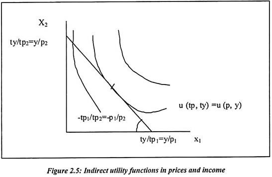
The utility maximization bundle can be written as x (p, y). The level of utility maximization is chosen at highest level by the consumer’s budget constraints. It is facing price p and income y. For group of individuals, the price and income gives different budget constraints. Such combinations give the different combination of indifference curves to consumers. The real value function shows the relationship between price, income and maximum value of utility.
It can be summarized by a real valued function as:
Above function is called as indirect utility function. When, u(x) is continuous u(x, y) is well defined for all p » 0 and y ≥ 0. This is because a solution to maximization problem exists. Consumer achieves maximum level of satisfaction subject to price (p) and income (y). It is true for all consumers. It is further written as
The u (p, y) gives the utility level of the highest indifference curve. Such utility function is shown in diagram. The consumer can reach at highest indifference curve with given prices p and income y. The price p and y is sufficient to guarantee that u (p, y) will be continuous in p and y on R”++ * R++. The continuity of u (p, y) follows positive prices. A small change in any of the parameters (p, y) fixes the location of the budget constraint. It will only lead to small changes in the maximum level of utility which the consumer can achieve.
Term Paper # 5. Expenditure Function:
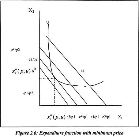
The expenditure function assumes that the prices of commodities are fixed. In order to achieve utility level, the consumer has to do certain expenditure at a given set of prices. For regular purpose, consumer’s come across the variety of commodities and prices. Most of the consumers have fixed level of income. Therefore consumer decides how much to spend on different commodities and achieve particular level of utility. Diagram shows that, all bundles of x require the same level of expenditure. The consumer faces the prices p = (p1, p2).
The iso-expenditure curves are defined implicitly by e = p1x1 + p2x2 for the different level of total expenditure where e > 0. Therefore there will be same slope —p1/p2. But different horizontal and vertical intercepts e/p1 and e/p2 respectively. Aniso-expenditure curve contains bundle and it is costing more. Consumer shifts upward on iso-expenditure lines. If we fix the level of utility at u, then the indifference curve u(x) = u. It gives all bundles which are yielding same level of utility to consumer.
The indifference curve u indicates e3 point. Money is insufficient at these prices to achieve maximum utility u. In the diagram, each of the curves e1 and e* has at least one point in common with u. Such point shows that the level of total expenditure is sufficient for the consumer to achieve utility u. Sometimes consumer does the regular minimum expenditure on various commodities to achieve fixed utility level. They also know that they cannot spend more of regular purchase of such commodities.
Expenditure function only explains that the consumer requires the minimum expenditure to achieve utility u. It is in the form of purchase of various goods and services. It is the lowest possible expenditure curve that still has at least one point in common with indifference curve u. The level of e* is the least cost bundle. It achieves utility u at prices p. we can call it as equilibrium point. It will be the bundle xh = (xh1 (p,u).xh2 (p,u)). The minimum expenditure u is required to achieve utility u at prices p by e (p, u). It means expected minimum utility is a function of price level. The level of expenditure is equal to the cost of bundles xh. It can be represented in terms of equation as e (p, u) = p1xh1 (p.u) p2xh2 (p, u) = e*
The expenditure function is the minimum value function. It is as follows:
Lowest level of expenditure is required to achieve utility level u.
Properties of Expenditure Function:
If u (.) is continuous and strictly increasing then e (p, u) defined into seven properties.
They are as follows:
Property 1:
Zero when u takes on the lowest level of utility in u:
The lowest value in utility is u (0). It is because u (.) is strictly increasing on Rh+. Consequently (p, u (o)) = 0 It is because x = o attain utility u (o). It requires expenditure of p0 = 0
Property 2:
Continuous on its domain Rn++* u:
Such property follows from the theorem of the maximum.
Property 3: For all p»0, strictly increasing and unbounded above in u:
Third property shown via additional hypothesis Xh (p, u) » 0 which is differentiate ∀p » 0, u > u (0) and that u (.) is differentiate with ∂u(x)/∂x > 0 ∀i on. We have assumed that the u (.) is continuous and strictly increasing. The p » 0 is the constraint and it is binding. For u (x’) > u, there is at ϵ(0, 1) which is close enough to 1. It is u (tx1) > u. Moreover u ≥ u (0) implies u(x1) > u (0) so that x1 ≠ 0.Therefore p.(tx1) < p.x1, because p.x1 > 0 when the constraint is not binding. There is strictly cheaper bundle that also satisfies the constraint.
If we write it in different way then:
The Lagrangian function is used for above function, therefore it is written as:
Now for p» and u > u (0), we have x* = xh(p, u)k”0
We need to solve equation 33. There is a λ* shown as:
The pi and ∂u(x*)/∂xi are positive. Due to hypothesis, the envelope theorem can be used to show that e (p, u) is strictly increasing in u. By the Envelope theorem, the partial derivative of the minimum value function e (p, u) with respect to u is equal to the partial derivative.
It is Lagrangian with respect to u and evaluated at (x*, λ*), hence:
Suppose, we hold for all u > u (0) and e (.) is continuous, we may conclude that for all p » 0, e (p, u) is strictly increasing in u on u (which includes u (0)). That e is unbounded in u and it can be shown to follow from the fact that u(x). It is continuous and strictly increasing.
Property 4:
Expenditure function is increasing in p:
Proof of above function is shown in the property 7.
The property 5:
Homogenous of degree 1 in p:
The proof of property is simple. The rise in price level (p) and income (y) is almost same. Therefore it is called as homogenous to degree one.
Property 6:
Concave in p:
Suppose p1 and p2 assumed as two positive price vectors. Let tϵ (0, 1) and pt = tp + (1-t) p2 be any convex combination of p1 and p2.
The expenditure function will be concave in prices if:
Now we will focus on what it mean to reduce the expenditure at given prices. Suppose particular x1 minimizes expenditure to achieve u when prices are p1. Similarly x2 minimizes expenditure to achieve u when prices are p2. Therefore x* is minimum expenditure to achieve u when prices are p2. The cost of x1 at process p1 must not more than the cost at prices p1 of any other bundle x that achieves utility u. Similarly, the cost of x2 at prices p2 must not more than the cost at p2 of any other bundle x, which achieves utility u if,
And
For all x that achieve u, the relations must also hold for x*. This is because x* achieves u as well.
To maximize expenditure to achieve u at given prices, we know that:
And
If t ≥ 0 and (1-t) > 0, we can multiply the first of these by t, the second by (1-t) and add them. If we then substitute from the definition of pt, we obtain,
In the above equation, left hand side is a convex combination of the minimum levels of expenditure. It is necessary at prices p1 and p2 to achieve utility u. The utility u must be constant at change in price. The right hand side is the minimum expenditure needed to achieve utility u at the convex combination of those prices.
Equation (37) explains that:
We intended to show from the previous equations is that such function is concave in p.
Property 7:
Shepherd’s Lemma:
e (p, u) is differentiable in p at (p0,u0) with p0 » 0 and
In order to use the above property, we can use the Envelope theorem. But now we differentiate it with respect to pi. It gives us following equation.
It is required because xh (p,u) ≥ 0. It is also possible to prove property 4. All the properties of the expenditure function are equally important and they help us to understand expenditure function in detail.
Expenditure Minimization Problem:
Every consumer tries to minimize total expenditure to increase utility. Sometimes consumer prefers substitutes to reduce expenditure. Most of the substitutes are available at lower price. The Expenditure Minimization Problem (EMP) explains the price and utility function. It, is explained as p » 0 and u > u (0).
There are unlimited wants for every consumer. It is explained because the minimum level of wealth is required to achieve utility u. Sometimes, it is used as the cutoff point to achieve minimum utility out of wealth. We can observe such cut off point for every family. It is an efficient use of the family’s purchasing power while reversing the roles of objective function and constraint.
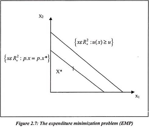
We assume that u (.) is a continuous utility function. It is representing a locally not satiated. Preference relation ≥ defined on the consumption set RL+. Above figure 2.7, shows that the optimal consumption bundle x* is the least costly bundle. It still allows the consumer to achieve the utility level u. Consumer gets maximum satisfaction with desired bundle of goods.
The geometric point of view, it is the point in the set {xԑRL+: u(x) ≥ u}. It lies on the lowest possible budget line associated with the price vector p. It is shown in the figure as x* point. If we assume that u (.) is a continuous utility function representing a locally non satiated preference relation ≥ defined on the consumption set x = RL+. The price vector is P.
Therefore:
1. If x* is optimal in the utility maximization problem when wealth is w > 0, then x* is optimal in the EMP when the required utility level is u(x*). The minimized expenditure level in the EMP is exactly w. Sometimes consumer cannot do the expenditure which is above his/her wealth.
2. Suppose x* is optimal in the EMP when the required utility level is u > u (0) then x* is optimal in the UMP when wealth is p.x*.
The minimized utility level in this UMP is exactly u.
If we want to prove the above proposition then, it can be shown as follows:
(i) Suppose x* is not optimal in the EMP with required utility level u(x*). Then there exist an x’ such that
By local non-satiation, we can write that x” is very close to x’. It also means u(x”) > u (x’) and p.x” < w.
Above notation implies that x” ϵBpw and u(x”) > u(x*). It is contracting the optimality of x* in the UMP. The x* must be optimal in the EMP when it required utility level is u(x*).The minimized expenditure level is p.x*. The x* solves the UMP when wealth is w. In Walra’s law, we have p.x*= w.
(ii) If u > u (0) and x* ‘”0; hence p.x* > 0.
If x* is not optimal in the UMP when wealth is p.x*. There exists an x’ such that u (x’) > u(x*) and p.x’ ≤ p.x*. If we consider bundle x”= ∝ x’ where ∝ϵ (0, 1). Here x” is a scaled down version of x’ through continuity of u (.), if ∝ is close enough to 1, then the u(x”) > u(x*) and p.x” < p.x*.The above notation contradicts the optimality of x* in the EMP. Therefore, x* must be optimal in the UMP when wealth is p.x*.
The maximized utility level is therefore u(x*). The required utility level is u, then u(x*) = u. According to utility maximization problem when p » 0. The solution to the EMP exists under general conditions. The constrained set needs to be non-empty. It means u (.) must attain values at least as large as u for some x. The condition will be satisfied for any u > u (0) if u (.) is unbounded above.
Term Paper # 6. Measures of Risk Aversion:
We are giving various axioms which are satisfying the consumer’s choice behavior. We can find a representation of utility that has the expected utility property. The consumer always gamble and his behavior is to more utility through prize. Therefore we need to do particular representation of his utility function for money. For example, to compute the consumers’ expected utility of a gamble, we have taken the simple probability as, p 0 x ⊕ (1-p) 0 y. Now we can present it in terms of utility function as Pu(x) + (1-p) u(y).
The consumers prefer to get the expected value of the lottery. The utility of the lottery u (p 0 x) 0 y, we just look it in another way as pu(x) + (1-p) u(y).
The consumers prefer to get the expected value of the lottery. The utility of the lottery u (p 0 x ⊕ (1-p) 0 y) is less than the utility of the expected value of the lottery px + (1-p) y. Such behavior is called risk aversion of consumer. There are two types of consumers. They are risk averse and risk lovers. Suppose a consumer who is risk loving; then he prefers a lottery to its expected value. The preferences for such consumer are different. Their value judgments for winning different lotteries are different. Concavity of the expected utility function is equivalent to risk aversion.
A risk-averse agent decides how to allocate his total wealth between investment in an asset with stochastic return (the risky asset) and an asset with deterministic return (the safe asset), so as to maximize the expected utility of return. If the return on the risky asset is less than that on the safe asset, ‘lie agent concentrates all his investment in the safe asset. On the other hand, if the mean return on the risky asset is greater than the safe return, the agent invests a positive fraction of his wealth in the risky asset.
Now, it is convenient to measure risk aversion in the following paragraph. The more concave is the expected utility function, then more the risk averse consumer. The graph of this utility function in this region must lie below the function. In order to normalize the second derivative we need to divide it by the first, we get a reasonable measure. It is known as the Arrow-Pratt measure of (absolute) risk aversion.
A gamble now by pair of numbers (x1, x2) where the consumer gets x1 if some event (E) occurs and x2 if event does not (E) occurs. We define the consumer’s acceptance set consists of both expectations. It is simple probability function. Consumer plays this gamble or it is the set of all gambles. The consumer would accept at an initial wealth level w. We assume that consumer buy lottery from his wealth. If the consumer is risk averse, the acceptable set will be a convex set. The boundary of this set and the set of indifferent gambles can be given by an implicit function x2 (x1).
If the consumer behavior can be described by the maximization of expected utility, then x2(x1) must satisfy the identity.
It is represented as follows:
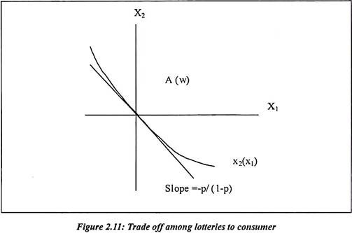
The slope of the acceptance set boundary at (0, 0). It can be found by differentiating this identity with respect to X1 and evaluating this derivative at X1 = 0.
Suppose we solve the above equation for the slope of the acceptance set, and then we find it as follows:
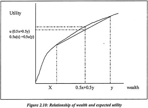
Figure 2.10 shows that the expected utility from both the lotteries 0.5u(x) + 0.5u(y) is equal. If we compare it with u (0.5x + 0.5y) then such utility is slightly more than the equal probability of x and y.
Utility of x and y is different. In terms of wealth, the utility of the y lottery is much more than the x lottery. It is the consumer who decides how to choose the two lotteries.
Figure 2.11: Trade off among lotteries to consumer Figure 2.11 shows that the slope of the acceptance set at (0, 0) and it gives odds. At the same time, it gives us the nice way of drawing out probabilities. We need to find the odds at which a consumer is just willing to accept a small count on the event in question. We can prove this with the help of two consumers and probabilities. Suppose there are two consumers with identical probabilities on the event E. we can further say that consumer i is more risk averse than consumer j.
If consumer i’s acceptance set is contained in consumer j’s acceptable set then this is global statement of risk aversion. It means that consumer j will accept any gamble that consumer i will accept. Suppose if we put our self in gambles then we get a more useful measure. Consumer i is locally more risk averse than consumer j then i’s acceptance set is contained in j’s acceptance set in a neighborhood of the point (0, 0).
By differentiating the identity one more with respect to x1 and evaluating the resulting derivative at zero, we find the following equation:
We can use the fact that x’2(0) = -p/ (1-p), we have:
Above equation is a proportion of the Arrow⎯Pratt measure. It is of local risk aversion which is already defined in above paragraph. A consumer j will take more risk with small gambles than agent i. But is only possible when ‘i’ have a larger Arrow-Pratt measure of local risk aversion. Risk aversion has many applications. Consumer always reduces the risk to improve economic gains.
