Here is a term paper on the ‘Production Function’ for class 9, 10, 11 and 12. Find paragraphs, long and short term papers on the ‘Production Function’ especially written for school and college students.
Term Paper on Production Function
Term Paper Contents:
- Term Paper on the Introduction to Production Function
- Term Paper on the Inputs to Output Function of a Firm
- Term Paper on the Technology Specification in a Firm
- Term Paper on the Input Requirement Set
- Term Paper on the Transformation Function
- Term Paper on the Monotonic Technologies
- Term Paper on the Convex Technology
- Term Paper on the Regular Technology
- Term Paper on the Cobb Douglas Technology
- Term Paper on the Leontief Technology
- Term Paper on the Variation in Scale
- Term Paper on the Homogenous and Heterogeneous Production Function
- Term Paper on the Duality of Cost and Production Function
- Term Paper on the Michale Kalechi Theory
- Term Paper on the Neo Keynesian Model of Distribution (Kaldor Model)
1. Term Paper on the Introduction to Production Function:
ADVERTISEMENTS:
Every firm produces different kinds of output. But while producing output firms have objectives of maximizing profit and reducing costs. For reducing costs, firms are using number of techniques. Sometimes labor insensitive and sometimes capital intensive techniques are used for production. Firms always produce output with maximum capacity. The wage of the workers, interest payment, increases the cost of production.
Firms increase revenue by increasing the sale of products. But the optimum production point is planned by each firm which gives higher profit. All the factors of production are utilized in a best manner to maintain maximum profit. For maximum profit, firms’ uses number of alternative methods of production on regular basis. Firm keep the production constant but it used the number of techniques to reduce different costs.
2. Term Paper on the Inputs to Output Function of a Firm:
Every firm uses inputs and produces output. Such inputs used in production function are labor, machinery, land etc. From the available resources, firm produces the maximum quantity of goods. It is also called as Production Possibility Frontier (PPF). Such PPF shows the different combinations of the inputs to output. The combination of production function is changing with different inputs. The time factor is also included in production function.
ADVERTISEMENTS:
It means the time dimension of specific inputs used in output. The production possibility frontier differs in terms of nature of output. Some commodities required different proportions of capital and labor. Some production functions have the same proportion of labor and capital. Some production functions required maximum labors where as some production functions require more capital. It is the firm, which decides the replacement of labor with capital.
Most of the time such replacements of factors of production are depending on factor rewards and endowments. In labor abundant region, more labor intensive goods are produced. At the same time, capital intensive goods are produced in developed countries. But in any production function, capital and labor intensive techniques are used.
3. Term Paper on the Technology Specification in a Firm:
In specification of technology, we have assumed that there is only one firm. Such firm produces n goods from available inputs. Most of the production of goods required some amount of labors and capital. The production plan is prepared by each firm. Such production plan of firm consists of use of inputs and production of output. Firm uses Yij units of input and produces Yj output in particular time.
ADVERTISEMENTS:
The net output of good j is given as:
If j is positive then the firm produces more of good j that it uses as input. It is vis-a-vis when firm uses better j than it produces output. The production plan of any firm is a vector Y in Rn. The Yj is negative if the jth good serves as a net input and positive if the jth good serves as a net output. The production possibility set is the technologically feasible production plan. It is denoted by Y and a subset of Rn. The Y set is a production plan where all inputs and output pattern described.
Every firm has two types of production function. First is the conventional production function and secondly the new or innovative production function. The innovative production function uses the new technologies and professional skilled manpower. Such technologically production function changes in short term. There is no fixed market for such goods. It is a trend or fashion of particular products. In globalization era, due to competition, firm uses the innovative production function to sustain in market.
In the short run all the factors of production are fixed. The technology set is fixed therefore only conventional production set is possible. Firm cannot take decision to hire more capital and skilled manpower. But in the long run, such factors may be variable in their nature. Therefore firms ‘technological possibility set may change. Firm take decision about the different factors of production and become competitive in the market. Firm plans a dominant strategy in the long term to increase the market share.
In the short run, the production function is denoted as Y (Z). It consists of all feasible net output bundles consist with the constraints level Z.
In the short run, suppose the factors are fixed then it is written as:
Where, Y (z) is a subset of Y and it consists of all production plans which is more feasible.
ADVERTISEMENTS:
ADVERTISEMENTS:
4. Term Paper on the Input Requirement Set:
Sometimes firm produces only one good from available inputs. The net output is (Y-X). Here X is vector of inputs and produce Y units of output. In the garment units, firm prepare a shirt from the available cloth.
For such production, the firm’s input requirement set is given as:
ADVERTISEMENTS:
The input requirement set is the set of all input bundles. Such bundles produce at least Y units of output. But firm also uses the land and labor in production function which is not taken into consideration at this point.
Isoquants:
The iso-quants are the production plan and possibilities of a firm.
It is defined as:
ADVERTISEMENTS:
The iso-quants are the given bundles that produce exactly Y units of output. Sometimes inputs combinations are changed in production function but output remained kept constant.
Short Run Production Possibility Set:
As we have pointed out that, in the short run production function is fixed.
If firm uses some proportion of labor and capital then it is written as:
ADVERTISEMENTS:
Where
K = Amount of capital used in production function
L: Amount of labor used as input in production function
It is an example of short run production possibility set. In the above production function, more amount of capital is used as compare to the labor.
5. Term Paper on the Transformation Function:
ADVERTISEMENTS:
A production plan Y in y is technologically efficient. Suppose there is no y’ in Y then Y’ > y and Y’ = y. A production plan is efficient if there is way to produce more output with the same inputs or to produce the same output with less input. It is also called as the efficient production function. Every firm prefers only efficient production function.
The transformation function can be written as:
Where T (y) = 0, it is possible when y is efficient. The production function picks out the maximum scalar output as a function of the inputs. The transformation function picks out the maximal vectors of the net output.
Activity Analysis in Production Function:
In activity analysis, we need to assume that there are two inputs in production function. Such inputs are required in production function. The output is produced using the factor inputs ⎯ labor and capital. The two different factors of production perform two different activities and the output is produced. Labor and capital are used in different proportion in production function. The labor does the labor intensive tasks whereas the capital does capital intensive tasks.
ADVERTISEMENTS:
From both the factors of production, output is produced. The labor intensive tasks are not possible by using more capital. We assume that the labor intensive tasks are specific in their nature. The capital intensive techniques use more machinery where labors are used for supervision or quality control. Sometimes more machines can produce more output. But sometime quality of production matters.
In the labor intensive techniques, two units of labor and one unit of capital is used to produce one unit of output. For example in garment unit, a machine is required for two workers. They perform activities such as swing and cutting of cloths. At the final stage, one worker can produce a shirt by joining different parts.
In the capital intensive technique, there are two units of capital and one unit of labor is used. In order to take print of a draft, a computer and printer is required. Such units are capital intensive units. One unit of labor is enough to take a print of a draft. But without printer, print of draft is not possible. In the modern world, firms produce number of goods with different combinations of labor and capital. There are number of possibilities of firm’s production set. The production possibility set implies two different set of production.
We can define Y as set of combinations; it is defined as follows:
Now if we assume that the firm is using the input requirement set. Such set can be written as follows, V (Y) = {(10, 20), (20, 10)}. Here the input required for production of goods is represented in to 2 subsets. Some time, the production of Y requires different combinations of inputs.
ADVERTISEMENTS:
We can write the possible combination as follows:
Equation shows that there are two subsets and possible production function.
Suppose we write further it as:
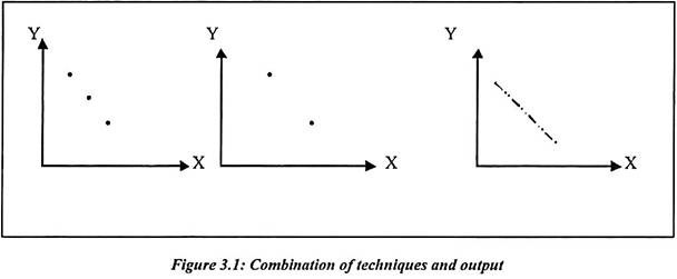
Now, the use of technique A which will require (y, 4y) input of two factors of production. Secondly, B type of technique required (4y, y) input of factor of production. Such technique and combinations are presented in the figure 3.1.
It is assumed that firm will either use technique A or technique B and output will get produced. Such output is explained as Y. The Y set is now explained different from the previous explanation.
It is given in the following form:
In the above set, there are different combinations. The last combination explains that (8, 8) can produce one unit of output.
6. Term Paper on the Monotonic Technologies:
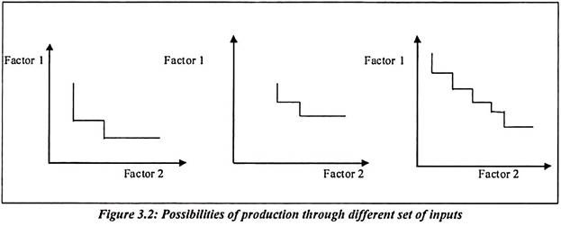
We have different input vectors to produce the output. Their combinations can be changed. Suppose we assume that the input factors are (2, 4) to produce output in a given time. It is also possible to produce one unit of output from (6, 4) input at particular time. We can say that x is a feasible way to produce y units of output and x’ is an input vector. It is with at least as much as of each input. We further say x’ should be a feasible way to produce y. Therefore the inputs are required Monotonic to produce output.
If x is in V(Y) and x’ > x then x’ is in V(Y).The above possibility is depicted in the figure 3.2
In above production function, we assume that y is in Y and Y < y. Now y’ must also be in y. Similarly, if y’ < y, it explains that every component of vector y’ is less than or equal to the corresponding component of y. The production plan represented by y’, it produces an equal or smaller amount of all output by using at least as much of all inputs as compared to y. Hence it is natural to assume that if y is feasible than y’ is also feasible.
7. Term Paper on Convex Technology:
In the convex technology, we need to assume actual output of commodity. Suppose we produce 100 units of output of any commodity. If we multiply the vectors (1, 2) and (2, 1) by 100 then we will get the following identity. At this point, we should be able to replicate what we were doing before and produce 100 times as much. In the possible situation, production processes will necessarily allow for the replication. In the process of replication, we can explain that (100, 200) and (200, 100) are the V (100). Suppose we operate 50 processes of activity A and 50 processes of activity B. Then we can use 10 units of good 1 and 150 units of good 2 to produce 100 units of output. Hence (150, 100) should be in the input requirement set. We have another set of example.
We could operate 25 processes of activity A and 75 processes of type B. It implies that 0.25 (100,200) + 0.75 (200, 100) = (75, 225) It should be V (100).
There is probability function as follows:
t (100, 200) + (1-t) (200, 100) = (100t + 200 (1-t), 200t + (1-t) 100)
It should be v (100) for t = 0.01, 0.02…………,
Now t is a fraction between 0 and 1
Convexity:
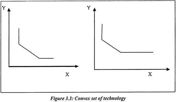
In the convexity of technology, if x and x’ are in V(y) then tx + (1-t) x’ is in v(y) for all 0 < t < 1 That is v(y) is a convex set. Such diagram is presented in figure 3.3,
If large amount is produced by a single firm then we can replicate small production processes. It appears that technology should be modeled as being convex. It increases with increase in production. If the scale of the underlying activities is large relative to the desired amount of output, convexity may not be a reasonable hypothesis. If one vector of inputs x produces y units of output then we might use other vector that is x which also produces y units of output. Here we might use x for half amount and x’.
It is common to assume that if y and y’ are both in Y, then ty + (1-t) y’ is also in Y for 0 < t < 1. In other words, Y is a convex set. It should be noted that the convexity hypothesis is problematic than the convexity of the input required set. The convexity production set implies convex input requirement set. Both are expected to be parallel with each other. Suppose the production set y is a convex set, then the associated input requirement set V(y) is also a convex set.
Proof:
We can represent proof in terms of simple probability function. We have (ty + (1-t)y, tx – (1-t) x’) in y. This is simply require that (Y-(tx+ (1-t) x)) is in y.
Above notation follows that if x and x’ are in V (Y). It explains that tx + (1-t) x’ which is in V (Y). It shows that V(Y) is convex. The convex input requirement set is equivalent to quasi concave production function. Now, V(Y) is a convex set. It is possible only if the production function F(x) is a quasi-concave function. The proof is given as V(Y) = x: f(x) > y, which is just the upper contour set of (x).
8. Term Paper on Regular Technology:
Few production functions required regular technology to produce output. Sometimes, it may be difficult to adjust output with new technology. In the regular technology set, the weak regularity condition concerning v(y) which is explained as regular technology. The v(y) is a closed non empty set for all y ≥ 0.
It is assumed that v(y) is nonempty set which requires that there is some conceivable way to produce any given level of output. Suppose we have a sequence (x1) of input bundles that can each produce y. This sequence converges to an input bundle x0. We can say that the input bundle in the sequence get arbitrary close to x0. Suppose v(y) is a closed set then this limit bundle x0 must be capable of producing y. It means input requirement set must include its own boundary. Sometimes it is true in production set.
Parametric Representations of Technology:
Firms use different ways to produce the given level of output. It depends on a choice of a firm about which inputs it has to use. These parametric technological representations should not necessarily be thought of as a literal depiction of production possibilities. The production possibilities sometimes viewed as engineering data. Such data describes the physically possible production plans. Firms regularly change the input set to produce same quantity of output.
Transformation Function:
In the transformation function, there is an n dimensional analog of a production function. Such function is useful in our study for general equilibrium theory. A production plan of any firm is y in Y. It is technological plan. Capital is used to increase the share of technology. Suppose there is no y’ in Y then y’ ≥ y can be possible option. Similarly y’≠ yi means a production plan is efficient if there is no way to produce more output with the same inputs. Alternatively it can be written as to produce the same output with less input.
We often assume that we can describe the set of technologically efficient production plan by a transformation function. It is written as T: Rn → R where T(y) = 0
Suppose y is an efficient, then the production function picks the maximum scalar output. It is a function of the inputs. The transformation function picks out the maximal vector of net output.
In terms of Leontief technology, the transformation function can be written as follows:
9. Term Paper on the Cobb Douglas Technology:
In Cobb-Douglas technology, the production function is defined in terms of technology set. Now all the competitive firms use maximum technology in their production function.
If we assume that the parameter which 1 < a < 1 then the Cobb Douglas technology is defined as follows:
Above equation shows the possible production, quantity of inputs, technology set with firm.
Leontific Technology:
Let a > 0 and b > 0 are the parameter, then the Leontific technology is defined as:
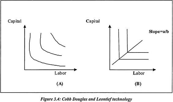
Such Leontief technology and Cobb-Douglas production function is explained in figure 3.4.
Figure 3.4(A) shows that Cobb-Douglas production function is convex in nature. In this figure, the labor and capital are indifferent. If labors proportion is reduced then automatically the proportion of capital rises. But the production will be indifferent at different points. Producer has more flexibility to adjusts both inputs and produce output. Such production function has general shape.
In the Leontief technology, both factors of production are used in same proportion. The change in factor may cause equal change in other factor. Sometimes they change in proportion with each other.
Figure 3.4A depicts production function of the Cobb Douglas technology which has general shape. They are isoquants of general production function. The panel B shows general shape of Leontief technology. Both factors of production are used in same proportion.
10. Term Paper on the Leontief Technology:
In some industries, the production is diverse in their nature. Therefore the production process may require the same factor proportion. Sometimes they remain constant. The delving of farm land is always not enough to add more workers. We must use the machine such as tractor to cultivate land. It means workers are complementary to cultivate land. But adding more tractors will not help to cultivate more land.
It will not increase the farm production. We need to increase the workers in proportion of plough. It means that the labor and capital must work together in a constant proportion. The proportion is one tractor for one worker. We have assumed that the worker know how to drive tractor.
In a particular production function Y = f (K, L). Such production function exhibits the fixed proportion function.
Property:
In order to produce a single unit of output, we need V units of capital and U units of labor. There is no flexibility in technique here. The co-efficient V and U are the fixed input requirement in order to produce a single unit of output. Suppose to produce Y units of output then we need VY units of capital and UY units of labor.
In other words,
It is the capital requirement and
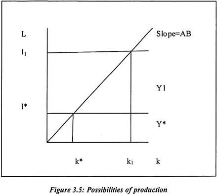
Above equation shows the labor requirement. If we combine two equation then the result is presented as follows and it is the only technique available as L/K = U/V. Labor to capital ratio is nothing but the unit of capital to the unit of labor. The implied L shape of iso-quant of such a production function is shown in the following figure 3.5.
Leontief Iso-Quants:
The Leontief iso-quants are explained with no substitution effect.
Such function for a no substitution case can be written as follows:
Above production function is referred as a Leontief production function. Such production function is introduced by Wassily Leontief in 1941. Such production function is used widely in technology set. Production possibility set in terms of Leontief technology is explained as follows. Let a > 0 and b > 0, both are the parameters in this function.
Then the Leontief technology is defined in the following manner:
Input Requirement Set:
Firm produces the output but it uses the input set. We can right it as the output in a function of input. The net output bundle is (y-x). In this function x is a vector of inputs that can produce y unit of output. Now, we can define a special case of a restricted production set. The input required set can be written as,
Above function explains that the input requirement set is the set of all input bundles. Such bundles produce at least y units of output. We can take a note that the requirement is defined differently. In production possibility set, the measured inputs are explained as the positive rather than negative numbers.
Such numbers and functions are explained in terms of Leontief technology set as follows:
In terms of the production of commodities, one can define the Iso-quants as follows:
The iso-quant shows all input bundles that produce exactly y units of output.
The Iso-quant in terms of Leontief technology is defined as follows:
Production function of a firm is defined differently. Suppose the firm has only one output, we can define production function in different way.
It is the maximum output associated with x in y.
Production function in terms of Leontief technology is defined in following equation:
It is most widely used production function.
11. Term Paper on the Variation in Scale:
In the variation of scale, we need to understand that the response to output to changes in inputs. Here, the change in any input can arise from the two basic points. Firstly, the change in the scale of production can take place by varying all inputs in same proportion. Secondly the change in relative input proportion can take place.
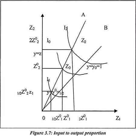
Figure 3.7 shows movements along the OA and OB points. The movement from one point to another point is explained in the following way. If we consider y point then the variation in y with scale parameters is with proportion. It is kept as constant.
The value implied by the initial z by the elasticity of scale is written as follows:
Alternatively, it can be written as
Suppose that E > 1 then it shows the increasing returns to scale. At the same time, if E = 0 then it shows the constant returns to scale. We can observe, E < 1 which means the decreasing returns to scale.
Since
∂y/∂s depends on the input mix. The returns to scale for production function may depend on the input mix and s. In figure 3.7, I0 and I2 iso-quants show constant returns to scale. The rays along OA and OB shows the increasing returns to scale.
12. Term Paper on the Homogenous and Heterogeneous Production Function:
We have seen that the production function is homogenous to degree one. Suppose we multiply all input by s then it leads to increase in output by factor st.
Suppose f (SZ) = Stfi (Z)
The production function is homogenous of degree t. In the production function T = 1. The production function is linear homogenous.
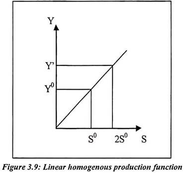
The homogenous production function of degree 1 is defined as:
The above linear homogenous function is equal to 1. It is also written as t = 1. The linear homogenous function has constant returns to scale. The constant returns to scale have all input combination.
In the above equation, two sides of equation must be equal. If we take a partial derivative of left hand side then
The partial derivative of right hand side is Stf(z), we have fi(sz) s = stfi(z).
It can be written alternatively as:
Above function is homogenous of degree t. It has partial derivatives which are homogenous of degree t-1.
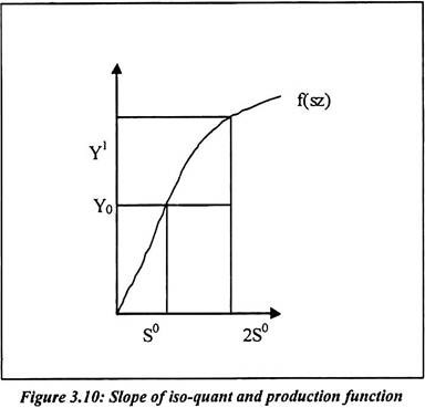
We have assumed that t = 1. It is linear homogenous function. Such marginal product is independent of scale. The slope of iso-quant at
The equation 42 holds for the all s which is homogenous. The derivative of left hand and right hand side of the equation (42) with respect to two must be s. The left hand side of equation (42) is
Such equation is derived from the equation 42. The right hand side of equation (42) is written as Tst-1f(z). Such function is homogenous to degree t.
13. Term Paper on the Duality of Cost and Production Function:
In a given a cost function, we can solve for a technology set. Such function can generate the cost function. This means that the cost function contains essentially the same information that the production function contains. The concept defined in terms of the properties of the production function which has a duel definition. It is in term of the properties of cost function and vice versa. This general observation is known as the principal of duality. Such principal is broadly defined as A set VO(y) which is an outer bound to the true input requirement set V(y).
In a given data (Wt, Xt, Yt), VO(y) is defined to be as follows:
Above equation is a straight forward to verify that VO(y) is a closed monotonic and convex technology.
Such equation contains any technology that could have generated the data (Wt, Xt, Yt) for t = 1…………… T
If we observe choice for many different factor prices then it seems that VO(y). In some sense, it should “approach” the true input requirements set. In order to make this precise, the factor prices vary over all possible price vector w ≥ 0.The natural generalization of Vo becomes as
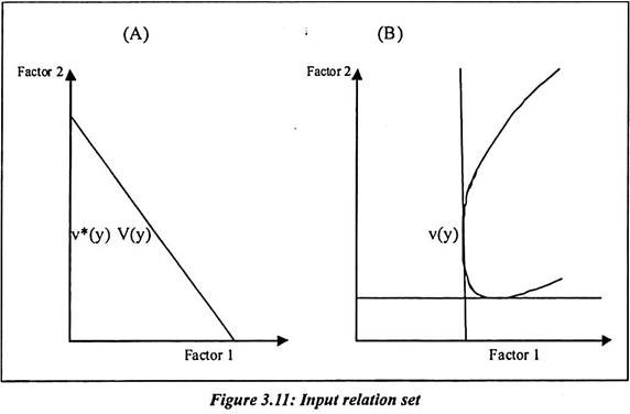
In the equation, the relationship between v*(y) and the true input requirement set V(y) is in general v*(y) will strictly contain v(y).For example in following figure (A) the left hand side area cannot be ruled out of V*(y) since the points in this area are satisfying the condition that wx ≥c (wy).
The relationship between v(y) and v*(y) is important. In the diagram, v*(y) will strictly contain V(y).
The same is true for figure 3.11(B). The cost function can only contain information about the economically relevant sections of v(y).Factors that could actually be the solution to a cost minimization problem; they could be conditional factor demands.
If we assume that technology is convex and monotonic, it is proved as follows:
In this case v*(y) will be equal to V(y). This is because in the convex, monotonic case, each point on the boundary of V(y) is a cost minimizing factor. Thus the set of point is where wx ≥ c (w, y). For all w ≥ 0, it will precisely describe the inputs requirement set more formally. Suppose, we assume that V(y) is a regular, convex, monotonic technology, then V*(y) =V(y). The proof is given as follows. From the above equation, we know that V*(y) contains V(y), so we have to show that if x is in V*(y) then x must be in V(y).
We can say that X is not an element of V(y).Since V(y) is a closed convex set satisfying the monotonically hypothesis. We can apply a version of the separating hyper plane theorem to find a vector. The W* ≥ 0 is because w*x < w*z for all z in V(y). Let us assume that z* be a point in V(y). It minimizes cost at the price w*.Now we have w*x < w*z*= C (w*, y). But we cannot define x is in V*(y). It is according to the definition of v*(y).This proposition shows that if the original technology is convex and monotonic then the cost function associated with the technology which can be used to completely reconstruct the original technology.
Suppose we start with some technology V(y), which may be possibly not convex. We find it is cost function c (w, y). Therefore it generates V*(y).We find cost function c (w, y) and then generate v*(y).We know from the above results v*(y) will not necessarily be equal to v(y), unless v(y). It is because the convexity and monotonicity properties. However, we need to define it differently as
It means X is in V*(y), when C (w, y) equals c*(w, y). It follows from the definition of the function that C*(w, y) = C (W, Y).
Such theorem is proved as follows:
It is easy to see that c*(w, y) ≤ c (w, y) since V*(y) always contains V(y). The minimal cost bundle in V*(y) must be at least as small as the minimal cost bundle in V(y).Suppose that for the same price w’, the cost minimizing bundle x’ in V*(y) has the property that
W’x’ = c*(w’, y) < C (w’y).But this cannot happen since by definition of V*(y),
This preposition shows that the cost function for the technology V(y) is the same as the cost function for its convex V*(y).
From the above discussion, we can explain that a given cost function, the input requirement set is v(y*). The original technology is convex and monotonic then the constructed technology will be identical. It will be with the original technology. Suppose the original technology is non-convex and non-monotonic, the constructed input requirement will be a convexities monetized version of the original set. The constructed technology will have the same cost function as the original technology.
14. Term Paper on the Michale Kalechi Theory:
In advanced microeconomic, the theory of Michale Kalechi is well known. The theory states that profit share is a function of degree of monopoly power of firm. That is
Where
∏b = Profit share of firm
δm = Degree of monopoly to firm
In a capitalist economy, the production capacity of individual firm is important. The actual production may increases or decreases but the capacity of firm does not change in long term. Therefore the excess capacity is a normal feature of the capitalist economy. As a consequence of this, the production decreasing or remain constant. The price of commodity is determined by the full cost principle. The prime cost is defined as the cost consisting of wages to manual worker plus cost of raw material.
The mark up pricing is defined as:
Where
Mp: Markup price
P = Profit and it is in the form of dividend
OC = It is an overhead cost and it is consists of interest, depreciation and salaries.
The above formula of markup pricing can be modified for single monopoly firm as follows:
Where
P = Price
K = Mark-up price
AVC = Average variable cost
The prime cost is defined as follows:
Where
K: Mark up price/prime cost
Ap: Aggregate proceed’
Apc: Aggregate prime cost
Where
K: Mark up price
W: Wage bill
R: Raw material cost
O: Overhead cost
E: Entrepreneur income
If we rearrange above equation then
From the above equation we have:
In the above equation, left hand side of equation represents sum of overhead and profits. We can assume that A is a value added by the production process.
We have substituted (O+E) from the above equation
We can divide above equation by W from both sides
Taking the reciprocal effect from the above equation
We have divided by W to above equation, therefore
It is a ratio of cost of raw materials to the wage bill. Above equation indicate that the share of wages in national income is function of two variables k and j. Under pure competition P = AC = MC.
Suppose P = AVC then K = 1
If the market deviates then pure competition is k > 1. In perfect competition, there is gap between the price and marginal cost. It will further lead to increase in the k. Now k represents the degree of monopoly in the market. The share of the wages in national income is higher than the monopoly power is greater. At the same time R/W = j is low. It is a ratio of cost of raw material to the wage bill.
Criticism:
Michel Kalechi model is criticized on various points. According to Kalechi there is growth of industry in the long term. It affects capital in the long term. It will reduce the share of wages to national income. Such effect is observed for agriculture products than the manufacturing items. The wage bill and its share remain stable in the long term. Such theory is also criticized by Bauer. He has lump together the overheads and profits in his theory. The major limitation of this theory is that it explains the microeconomic phenomena. But it concludes the macroeconomic phenomena.
15. Term Paper on the Neo Keynesian Model of Distribution (Kaldor Model):
The Neo Keynesian model of distribution is the full fledge macro-economic model. Such model uses the concept of aggregate income, saving and distribution of income. This model assumes condition of full employment. It is an endogenously constant ⎯ given by the state of confidence in the economy and it is not determine by the distribution of income. There are two income categories that are wages and profit. Wages include payment to manual labor and salaries.
Profit of firm includes the returns to entrepreneur and income of permanently owner. The constant saving propensities are assumed in the model. It states that average propensity to consume of each group is same. However, the propensity to save out of profit is explained in the model. With assumptions, Kaldor proceeds to establish the consistency of the relative factors share and capital output ratio.
The model can be expressed using following symbols:
Where
y = Wage income
w = Wage bill
p = Profit
Y = S and
Where
S = Saving
Sp = Average and marginal propensity to save out of profits
Sw = Aggregate saving out of wage income sww
Now
Substituting equation (81) into 80
Dividing both side by Y
With the assumption Sp and Sw is constant share of profit in NI. It is direct function of share of lt in NI.
The important assumption is made where Sp > Sw. We have stated the equilibrium as I = S. Suppose the ratio of It to national income increases then the equality get disturb. But suppose investment (I) is not equal to saving(s) then the price will rise.
The steps are given as follows:
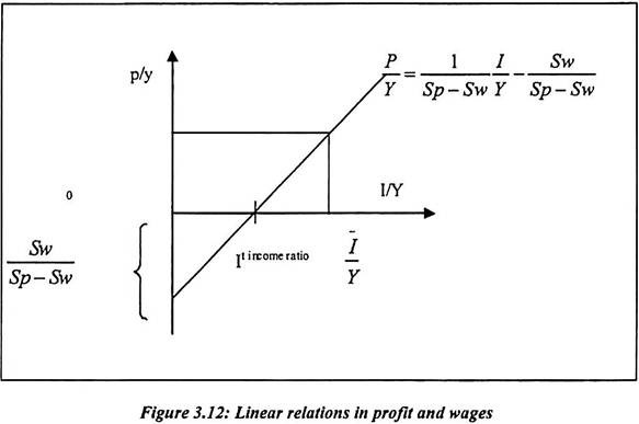
As I/Y increases then p also increases. It leads to increase in n/y but at the same time Sp > Sw where saving (s) increases. It increases till saving equals investment (S = I). The only way saving can be brought to equality with I1 is through a change in the distribution of income in favor of profit and away from wages. The mechanism explained above can be shown in graphical way in figure 3.12.
The above figure 3.12 depicts a linear relation between the rate of profit and the Rate of It. Any change in the rate of It leads to a corresponding change in the rate of profit. The rate of savings increases until It decreases. But then there is decrease in aggregate demand. It further leads to decrease in prices and increase in n. The model may be representing in slightly different way.
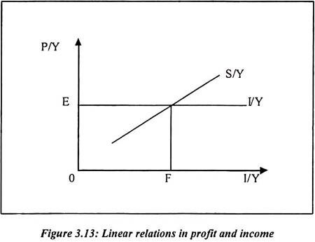
Since It is exogenous given and independent of P/Y. The ratio of I/Y is constant and it is given as horizontal line in figure. On the other hand Sp > Sy, therefore S/Y increases with P/Y. So that s/y function has positive slope. In the above figure, the ratio of I/Y = OF means ratio of P/Y = OE. Any increase in I/Y will increase the share of profit and lowers the share of income. On the other hand the net increase in aggregate propensity to save will increase with wage share. The stability of system depends on the relative saving propensity of worker and capitalists.
Equation 84 explains that-
Suppose (Sp ⎯ Sw) is positive, then very small infinitely change in I/Y will tend to produce large change in p/y. The system is stable if Sp = Sw, the system becomes explosive. Therefore it is necessary that Sp ≠ Sw and secondly Sp > Sw. If Sw = 0 the above equation becomes,
There are two interesting conclusions that emerge from the above discussion. Since, Sw = 0 it means people mostly spend all their earnings. Therefore average saving out of income may be positive. Secondly, since P = 1/Sp capitalist learn what they spend from their expenditure. This is because income of capitalist is directly from of their expenditure. An increase in expenditure of capitalist raises level of real profit by the extent of expenditure adopted for their propensity to save. Thus two basic features explain basic idea. The rate of It is a propensity to save out of profit.
