Theories of Business Cycles (With Criticisms) | Theories | Macroeconomics

In this article we will discuss about the theories for business cycles. Also learn about its criticisms.

Economists have observed business cycles (i.e., short-run economic fluctuations) for more than two centuries.

Here are some of the different approaches that have been proposed:

1. Monetary Theories:

These theories developed by R. G. Hawtrey and Milton Friedman attribute business fluctuation to the expansion and contraction of money and credit. In truth, the US recession 1981-82 was triggered when the Fed raised nominal interest rate to 18 per cent in order to fight inflation. According to these theories, monetary factors are the primary source of fluctuations in aggre­gate demand.

According to Hawtrey business cycles are a purely monetary phenomenon, which must, therefore, be controlled by regulating credit to wholesalers and retailers via the Bank Rate (or Discount Rate) and not by regulating public expenditure. He never contemplated di­rect control of the money supply as advocated by modern monetarists. But this is quite perfect keeping with the times because in the thirties monetary policy always meant rightly or wrongly a policy about the rate of interest rate and not a policy about money supply targets.

2. The Multiplier-Acceleration Model:

This model was presented by P. A. Samuelson in 1939. Samuelson proposed that exogenous shocks are propagated by the multiplier mechanism of Keynes (1936) along with a theory of investment called the acceleration principle, originally presented by A. Aftalion and then re­fined and modified by J. M. Clark in 1917. Samuelson’s model shows how the interaction of multiplier and accelerator can lead to regular cycles in aggregate demand. This model gener­ates internal cycles.

The Samuelson Model: Paul Samuelson was stimulated by Alvin Hansen to work out in rigorous form as early as 1939 what has become the best known of the multiplier-accelerator interaction models. We present it briefly before indicating some of its analytical limitations.

Samuelson’s model is a non-accelerator interaction model with both consumption and in­vestment endogenous and with both functions taking a dynamic form. The equations of the model are:

Equation (7.1) indicates that consumption is a linear function of income of the previous period. Investment, as equation (7.2) shows, is proportional to the change in the level of con­sumption between the previous and current period. Here v is the accelerator, i.e., the ratio of investment to the change in consumption. It is assumed to be positive.

It is also assumed that spending plans in period t are realised, so that the income definition is (7.3). In this model, which we may call no-policy model, government expenditure (G) is exogenous and constant. No attempt is made to use G as an instrument for controlling the time path of income. Substitut­ing for G, and I, from equations (7.1) and (7.2) in the income equation (7.3), we have the expression for Y_t.

This is a second-order difference equation-which, can easily be solved. The equilibrium level of income Y^e is found by setting for equilibrium Y_t =Y_t-1 = Y_t–₂ in equation (7.4), so that … (7.5)

……(7.5)

Investment is now entirely endogenous so that there is no I in equation (7.5). Equilibrium income is the product of exogenous expenditure and the multiplier. The reason for the equiva­lence is that in equation Y_t = Y_t-1= Y_t-2 which means (from equation (7.1) that C_t = C_t = C _t-1 with C constant, there is no induced investment (from equation (7.2).

In disequilibrium, however, consumption plans change as the multiplier effect of a change in exogenous expression works itself out. With C_t ≠ C_{t -1}, the multiplier-accelerator model displays several characteristics. Investment reacts to the change in consumption and the change in investment expenditure in turn feeds back, via income, to consumption.

There is an interac­tion between induced consumption changes and induced investment changes which gives rise to the possibility of cycles in the time path of income. We may now establish the conditions under which cycles will occur.

Equation (7.4) can be written as:

Here k is dependent on both b and v, as equation (7.9) shows. It will be found, therefore, the income path varies with different combinations of parameters b and v.

Because (7.9) is quadratic there is no single solution for k. There are two roots—k₁ and k₂— of equation (7.9), which are found from

The values of k₁ determine whether the system is stable and converges on Y_e, and whether the path towards, or away from, equation will be smooth or cyclical. Since k₁, and k₂ depend on b and v, the conditions for convergence and for cycles can be expressed in terms of b and v.

The outcome is a classification of all possible combinations of b and v, first into those producing cycles and those yielding smooth income paths; and second into combinations leading to con­vergence of equilibrium and those which produce explosive (divergent) income paths.

The requirement for cycles to occur is that

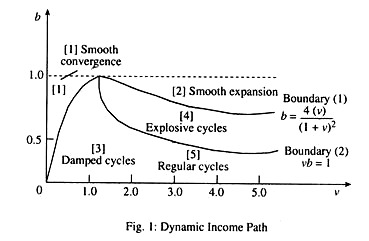
In Fig. 1 all combinations of v and b which are below boundary [1] meet this requirement and produce cycles. These on or above this boundary represent smooth growth or smooth de­cline of income.

The condition for the system to be convergent is that

vb < 1

In Fig. 1 the combinations above boundary [2] fail to satisfy this requirement and yield explosive income paths. Those falling on boundary [2] yield regular cycles and those below it yield convergent income paths.

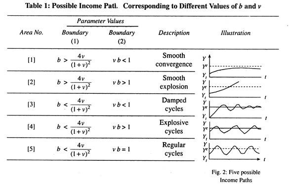
These two divisions create four areas of combinations of v and b, plus the special case of a fifth ‘area’ on the boundary [2], The characteristics of the resulting income paths following a disturbance from equilibrium are summarised by means of Fig. 2 and Table 1.

The condition for the system to be convergent is that

vb < 1

In Fig. 1 the combinations above boundary [2] fail to satisfy this requirement and yield explosive income paths. Those falling on boundary [2] yield regular cycles and those below it yield convergent income paths.

These two divisions create four of v and the special case of a fifth ‘area’ on the boundary [2]. The Characteristics of the resulting income paths following a disturbance from equilibrium are summarized by mean of Fig.2 and Table1.

In Table 1 the first column gives the number of the corresponding areas in Fig. 2. The second and third columns show the relationship of each area to the two boundary conditions. In the case of area [3], for example, both the conditions for convergence and that for cycles is met, and the result is damped (convergent) cycles as shown in words in the fourth column and diagrammatically in the fifth column. In these illustrative figures Y^e is the equilibrium income level and Y_t an initial disequilibrium income.

Criticisms:

There are four important limitations of the model as an explanation of the busi­ness cycle:

1. It is built on a very simple explanation of the determinants of aggregate demand since the expenditure sector used contains no monetary factors.

2. It does not impose any restrictions on variations in income and therefore in output. The combination of v and b determines the time path of aggregate demand, and the model assumes that none of the resulting demand levels exceed full employment output.

3. It produces symmetrical cycles, that is, cycles with upswings and downswings of similar duration.

4. It does not explain the trend of equilibrium income about which cycles may occur in practice because the equilibrium level of income is exogenous to the model.

Conclusion:

Nevertheless this Hansen-Samuelson model has had a great appeal for econo­mists, as offering a simple yet logical explanation of the essential mechanism of the business
cycle.

In fact, in an interesting experiment, G.H. Fisher showed how this cycle model would produce a synthetic ‘time series’ that looks quite convincing like the familiar series used to show the business cycle, and with no apparent tendency for the cycle to die out, even after several hundred successive periods.

3. Equilibrium Business Cycle Theories:

These theories developed by R. Lucas, R. Barro and T. Sargent claim that misperceptions about price and wage movements lead people to supply too much or too little labour, which leads to fluctuations of output and employment. One version of these theories suggests that unemploy­ment rises in recessions because workers, who are paid too high wages during recovery are reluctant to accept low wages.

4. Real Business Cycle (RBC) Theories:

Following the ideas of J. Schumpeter, E. Prescott, P. Long and C. Plosser hold that innovations or productivity shocks in one sector can spread to that rest of the economy and cause recessions and booms. In this new classical approach, cycles are caused primarily by shocks to aggregate supply, and not by changes in aggregate demand.

Supply Shocks:

Supply shocks occur when business fluctuations are caused by shift in aggregate supply. The classic examples were the oil crises of the seventies. Sharp increases in oil prices reduced aggregate supply, increased inflation and lowered output and employment. Thus, the RBC approach holds that business cycles are primarily due to changes in technol­ogy and does not invoke any monetary or demand-side forces.

In the RBC approach, shocks to technology, investment, or labour supply change the poten­tial output of the economy. In other words, they shift a vertical aggregate supply (AS) curve. These supply shocks are transmitted into actual output by the fluctuations of aggregate supply and are completely independent of aggregate demand (AD). Likewise, movements in the un­employment rate are the result of movements in the non-accelerating inflation rate of unemploy­ment (NAIRU) due to microeconomic forces such as the intensity of sectoral shocks or to tax policies or other regulatory measures.

A Retailed Discussion of Real Business Cycle:

RBC models view aggregate economic variables as the outcomes of the decisions made by individual agents acting to maximise their utility subject to production possibilities and re­source constraints.

As such these models have an explicit foundation in microeconomics. More explicitly, RBC models ask the following two questions:

(l) How do rational maximising individuals respond over time to changes in the economic environment?

(ii) What implications do these responses have for the equilibrium outcomes of aggregate vari­ables? Invariably RBC models address these questions in a general equilibrium Walrasian frame­work.

Two important features of RBC models are:

(i) Explanations for fluctuations in terms of shocks and

(ii) Propagation mechanisms through which the effects of shock are spread throughout the economy. RBC models emphasise real shocks mainly in the form of shock to technology, i.e., changes in the production function from period to period. More recently RBC models also emphasise changes in government purchases. Technology shocks change the amount that is produced from a given quantity of inputs and government purchase shocks change the quantity of goods available to the private economy for a given level of production.

Thus, we see that both types of shocks represent real as opposed to monetary disturbances. The transmission or propagation mechanism operates through inter-temporal substitution of labour. Accordingly this model allows for changes in employment by making household’s util­ity depend on both consumption and work.

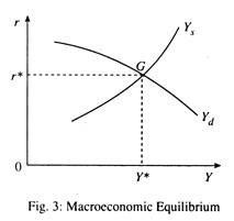
Let us now construct a simple RBC model.

The production function is

y_t = K_t^α(A_t L_t )^1-α

This represents labour augmenting technological progress. Labour and capital are paid their marginal product. Thus, real wage and real interest rate are written as

Let us now consider technology. This is written as

log A_t = A̅ + g_t + Â_t

Here g is the rate of technological progress. However, technology is subject to a random shock A_t. Now, this random shock is a first-order autoregressive process, i.e., A, = βA_t–₁ + ε_t, where ε_t has zero mean and constant variance. In other words goal ε_t represents white noise disturbances. (They are serially uncorrelated and random; ε_t’s have a constant mean, i.e., 0 and a variance, ε_t, is the random shock term).

Here β < 1 (if β > 1, the model would explode).

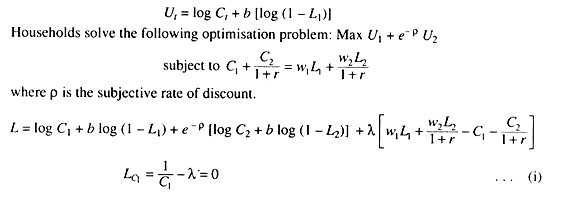
Let us now consider household’s optimisation goal from which we will derive the labour supply function. Let us suppose that each household has only one member and total time avail­able is one unit. For the sake of simplicity we choose a two-period optimisation framework. We consider the following utility function

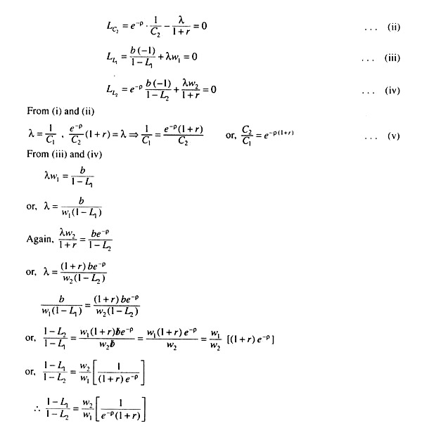
This equation implies that relative labour supply in the two periods responds to the relative wage as well as interest rate. If, for example, w₁ increases, the households increase first period labour supply relative to second period labour supply. Again a rise in interest rate leads to increase in first period labour supply relative to second period labour supply. These responses of labour supply to real wage and interest rate are known as inter-temporal substitution in labour supply. We know, from (v) above, that

From above it follows that a rise in interest rate reduces current consumption relative to future consumption.

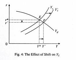
Let us now consider output supply function. If interest rate rises, work effort in current period goes up, leading to rise in output level. Now we consider aggregate demand. At any time t, aggregate demand is

AD _t = C_t (r) + I_t (r) + G_t C’_t<0, I_t< 0

If interest rate goes up, both current consumption and investment fall and thus aggregate demand is inversely related to interest rate. Let us suppose that aggregate demand increases. Out­put supply function moves to the right, as shown in Fig. 4.

Output increases from Y* to Y’ and interest rate falls from r* to r.

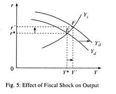
Fiscal Shock:

Here rises if Y_d shifts rightwards.

This implies that r rises.

This implies that L₁ rises and output supply rises.

The inter-temporal real wage ratio is

If w₁ or r rises, then L₁ increases, i.e., leisure falls and, therefore, labour supply rises.

Criticisms of Real Business Cycle Theory:

The real business cycle theory has been criticised on various fronts which we now proceed to explain.

First, the RBC theory stresses more on supply-side variables than on demand side vari­ables.

Second, the RBC theory assumes that output is always at its natural level. The theory does not make room for stickiness of wages and prices. It says that fluctuations in output are move­ments of the natural level. However, not all fluctuations in output are deviations from the natural level.

Third, it is hard to think of recessions as times of technological regress, times in which productivity and output both go down.

Fourth, technological progress results from many innovations, each of which takes a long time to diffuse throughout the economy. So it is not convincing that such process could gener­ate short-run fluctuations.

Finally, changes in money supply, which have strong effects on output in the real world, have no effect on output in RBC models.

So, the majority of economists do not believe that the RBC approach provides a convincing explanation of major fluctuations in output. But, the approach has proved useful and influential.