I. Rationalisation of the Sales Maximisation Hypothesis:
Baumol offers several justifications of sales maximisation as a goal of the firm.
The separation of ownership from management, characteristic of the modern firm, gives discretion to the managers to pursue goals which maximise their own utility and deviate from profit maximisation, which is the desirable goal of owners.
Given this discretion, Baumol argues that sales maximisation seems the most plausible goal of managers. From his experience as a consultant to large firms Baumol found that managers are preoccupied with maximisation of the sales rather than profits. Several reasons seem to explain this attitude of the top management.
ADVERTISEMENTS:
Firstly, there is evidence that salaries and other (slack) earnings of top managers are correlated more closely with sales than with profits.
Secondly, the banks and other financial institutions keep a close eye on the sales of firms and are more willing to finance firms with large and growing sales.
Thirdly, personnel problems are handled more satisfactorily when sales are growing. The employees at all levels can be given higher earnings and better terms of work in general. Declining sales, on the other hand, will make necessary the reduction of salaries and other payments and perhaps the lay-off of some employees. Such measures create dissatisfaction and uncertainty among personnel at all levels.
Fourthly, large sales, growing over time, give prestige to the managers, while large profits go into the pockets of shareholders.
ADVERTISEMENTS:
Fifthly, managers prefer a steady performance with ‘satisfactory’ profits to spectacular profit maximisation projects. If they realize maximum high profits in one period, they might find themselves in trouble in other periods when profits are less than maximum.
Sixthly, large, growing sales strengthen the power to adopt competitive tactics, while a low or declining share of the market weakens the competitive position of the firm and its bargaining power vis-a-vis its rivals.
The desire for a steady performance with satisfactory profits, coupled with the separation of ownership and management, tend to make the managers reluctant to adopt promising projects which are risky. The top managers become to a certain extent risk- avoiders, and this attitude may act as a curb on economic growth. However, the desire for steady performance has a stabilizing effect on economic activity.
In general, large firms have research units which develop new ideas of products or techniques of production. The application of these projects is spread over time so as to avoid wide swings in the economic performance of the firm. Baumol seems to imply that the risk-avoidance and the desire for steady growth of the large corporations-secure ‘orderly markets’, in the sense that they have stabilizing effects on the economy.
ADVERTISEMENTS:
II. Interdependence and Oligopolistic Behaviour:
Although Baumol recognises the interdependence of firms as the main feature of oligopolistic markets, he argues that in ‘day-to-day decision-making management often acts explicitly or implicitly on the premise that its decisions will produce no changes in the behaviour of those with whom they are competing . It is only when the firm makes ‘more radical decisions, such as the launching of a major advertising campaign or the introduction of a radically new line of products, that management usually does consider the probable competitive response. But often, even in fairly crucial decisions, and almost always in routine policy-making, only the most cursory attention is paid to competitive reactions’.
This attitude towards competitors attributed by Baumol to several reasons:
The complexity of the internal organisation of large firms renders decision-making a lengthy process: proposals originate from some sections, but final decisions are taken by top management after these proposals have passed through various levels of management and often from different departments. It is a characteristic inherent in the delegation of authority within the firm that each decision-maker will attempt to shift the responsibility on to others. Thus any reaction of competitors is bound to take place after ‘a considerable time lag’.
Large organisations work to a ‘blue-print’ which includes a variety of rules of thumb, which simplify complicated problems such as pricing, size of advertising expenditure, level of inventories. Prices are set by applying a standard mark-up to costs, advertising expenses are determined by setting aside a fixed percentage of total revenues, inventories are determined as a percentage of sales, and so on. Such rules of thumb clearly do not automatically take into account the actions of competitors, and the adaptation of the ‘blue-print’ of a firm to a new environment takes time.
The desire of top management for a ‘quiet life’ has led large enterprises to some tacit collusion firms depend on each other to behave in an ‘orderly’ way. They expect no ‘breach of etiquette’ in the established order in the industry as a whole. However, the above reasons do not imply that businessmen are completely indifferent to actions of competitors. In particular, being sales maximisers and growth seekers, they are very alert to any change in their share of the market. Top management will ignore competitors only to the extent that their actions do not encroach on the firm’s market and do not interfere with the desired rate of growth of the sales of the firm.
III. Baumol’s Static Models:
The basic assumptions of the static models:
1. The time-horizon of a firm is a single period.
ADVERTISEMENTS:
2. During this period the firm attempts to maximise its total sales revenue (not physical volume of output) subject to a profit constraint. The firm in these models does not consider what will happen in subsequent periods as a result of the decisions taken in the current period.
3. The minimum profit constraint is exogenously determined by the demands and expectations of the shareholders, the banks and other financial institutions. The firm must realize a minimum level of profits to keep shareholders happy and avoid a fall of the prices of shares on the stock exchange. If profits are below this exogenously determined minimum acceptable level the managers run the risk of being dismissed, since shareholders may sell their shares and take-over raiders may be attracted by a fall of the prices of shares.
4. ‘Conventional’ cost and revenue functions are assumed. That is, Baumol accepts that cost curves are U-shaped and the demand curve of the firm is downward-sloping.
We will examine four models:
ADVERTISEMENTS:
(1) A single-product model, without advertising.
(2) A single-product model, with advertising.
(3) A multiproduct model, without advertising.
(4) A multiproduct model, with selling activities.
ADVERTISEMENTS:
Model 1: a single-product model, without advertising:
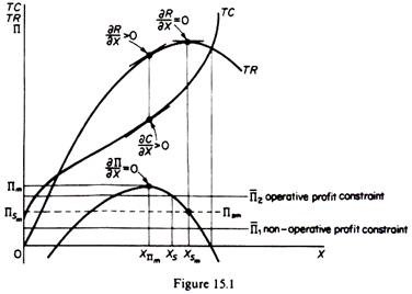
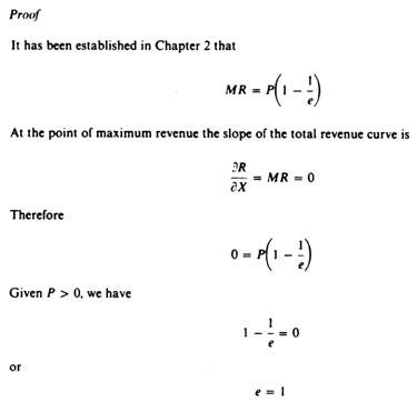
The total-cost and total-revenue curves under the above assumptions are shown in figure 15.1. Total sales revenue is at its maximum level at the highest point of the TR curve, where the price elasticity of demand is unity and the slope of this TR curve (the marginal revenue) is equal to zero.
Whether this maximum sales revenue will be realized or not depends on the level of the minimum acceptable level of profit which may act as a constraint to the activity of the firm. If the firm were a profit maximiser, it would produce the level of output Xnm. However, in Baumol’s model the firm is a sales maximiser, but it must also earn a minimum level of profit acceptable to shareholders and to those who finance its operations.
If the minimum acceptable level of profit is Π1, the firm will produce the level of output XSm which maximises its sales revenue. With this level of output (XSm) the firm earns profits ΠSm, which are greater than the minimum required to keep the stockholders (and other interested parties) satisfied. Under these circumstances we say that the minimum profit constraint is not operative.
ADVERTISEMENTS:
If the minimum acceptable profit is Π2, the firm will not be able to attain the maximum sales revenue because the profit constraint is operative, and the firm will produce Xs units of output, which are less than at the level XSm.
In summary… two types of equilibria appear to be possible one in which the profit constraint provides no effective barrier to sales maximisation (XSm units of output with a minimum acceptable profit of Π1), and one in which it does (XS units of output with a minimum acceptable profit of Π2)’. (W. J. Baumol, Business Behaviour, Value and Growth. The firm is assumed to be able to pursue an independent price policy, that is, to set its price so as to achieve its goal of sales maximisation (given the profit constraint) without being concerned about the reactions of competitors.
Provided that the profit constraint is operative, the following predictions of Baumol’s single-period model (without advertising) emerge:
The sales maximiser will produce a higher level of output as compared to a profit maximiser.
Proof
A profit maximiser produces the output XΠm defined by the equilibrium condition MR = MC or
ADVERTISEMENTS:
∂R/∂C = ∂C/∂X
Given that the marginal cost is always positive (∂C/∂X > 0) it is obvious that at the level XΠm the marginal revenue is also positive (∂R/∂X > 0). That is, TR is still increasing at XΠm, since its slope is still positive. In other words, the maximum of the TR curve (where its slope is ∂R/∂X = 0) occurs to the right of the level of output at which profit is maximised. Hence XSm > XΠm.
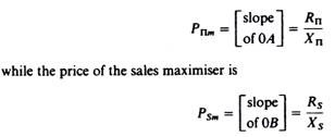
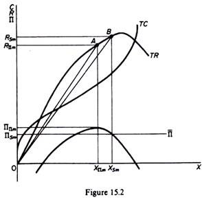
The sales maximiser sells at a price lower than the profit maximiser. The price at any level of output is the slope of the line through the origin to the relevant point of the total-revenue curve (corresponding to the particular level of output). In figure 15.2 the price of the profit maximiser is
It is obvious that (slope 0A) > (slope OB), that is, the price of the profit maximiser is higher than the price of the sales maximiser. The sales maximiser will earn lower profits than the profit maximiser. In figure 15.2 the profit of the sales maximiser is 0Πs, which is lower than the profit 0Πn of the profit maximiser.
The sales maximiser will never choose a level of output at which price elasticity (e) is less than unity, because from the expression
ADVERTISEMENTS:
MR = P (1 – 1/e)
we see that if ׀e׀ < 1, the MR < 0, denoting that TR is declining. The maximum sales revenue will be where |e| = 1 (and hence MR = 0) and will be earned only if the profit constraint is not operative. If the profit constraint is operative the price elasticity will be greater than unity.
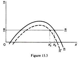
An increase in the fixed costs will affect the equilibrium position of a sales maximiser he will reduce his level of output and increase his price, since the increase in fixed costs shifts the total-profit curve downwards. Subject to the profit constraint, the sales maximiser will pass the increase in costs to the customers by charging a higher price.
This is shown in figure 15.3. The increase in fixed costs shifts the total costs upwards and the total-profits curve downwards (Π). Subject to the profit constraint Π, the firm will reduce its output (to Xs) and will increase its price.
This prediction is contrary to the traditional hypothesis of profit maximisation. A profit maximiser will not change his equilibrium position in the short run, since fixed costs do not enter into the determination of the equilibrium of the firm. So long as the fixed costs do not vary with the level of output (and provided that the increase in TFC does not lead the firm to close down altogether) the change in the TFC will not lead the profit maximiser to change his price and output in the short run.
ADVERTISEMENTS:
Baumol claims that firms in the real world do in fact change their output and price whenever their overhead costs increase. Thus he says that the sales-maximisation hypothesis has a better predictive performance than the traditional profit-maximisation hypothesis.
The imposition of a lump-sum tax will have similar effects. If the firm is a profit maximiser the imposition of the lump-sum tax will not affect the price and output in the short run the profit maximiser will bear the whole burden of the lump-tax. If the firm is a sales maximiser, however, the lump-tax will shift the total-profit curve downwards and, given the profit constraint, the firm will be led to cut its level of output and increase its price, thus passing on to the consumer the lump-sum tax. Baumol argues that firms do in fact shift the tax on to the buyers, contrary to the accepted doctrine about the ‘unshiftability’ of the tax.
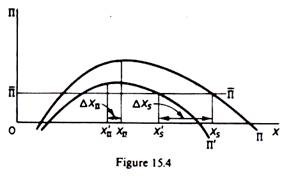
The imposition of a specific tax (per unit of output) will shift the profit curve downwards and to the left (figure 15.4). Given Π, the sales maximiser will reduce his output from Xs to X’s and will raise his price, passing the tax to the buyers (at least partly). The profit maximiser will also reduce his output (from XΠ to XΠ) and raise his price. However, the decrease in output will be larger than the decrease of the output of a profit maximiser.
A similar analysis holds for an increase in the variable cost. Both the sales maximiser and the profit maximiser will raise their price and reduce their output. The reduction in output, however, and the increase in price will be more accentuated for the sales maximiser, ceteris paribus. A shift in demand will result in an increase in output and sales revenue but the effects on price are not certain in Baumols model. Price will depend on the shift of the demand and the cost conditions of the firm.
Model 2: A single-product model, with advertising:
The Assumptions of the Model:
As in the previous model the goal of the firm is sales revenue maximisation subject to a minimum profit constraint which is exogenously determined. The new element in this model is the introduction of advertising as a major instrument (policy variable) of the firm. Baumol argues that in the real world non-price competition is the typical form of competition in oligopolistic markets. The model presented by Baumol treats explicitly advertising, but other forms of non-price competition (product change, service, quality, etc.) may be analysed on similar lines.
The crucial assumption of the advertising model is that sales revenue increases with advertising expenditure (that is, ∂R/∂a > 0, where a = advertising expenditure). This implies that advertising will always shift the demand curve of the firm to the right and the firm will sell a larger quantity and earn a larger revenue. The price is assumed to remain constant. This, however, is a simplifying assumption which may be relaxed in a more general analysis.
Another simplifying assumption is that production costs are independent of advertising. Baumol recognizes that this is an unrealistic assumption, since with advertising the physical volume of output increases and the firm might move to a cost structure where production cost is different (increasing or decreasing). But he claims that this assumption is simplifying and can be relaxed without substantially altering the analysis. (In fact Baumol relaxes this assumption, as well as the assumption of constant price in the mathematical presentation of his model; see below.) From the above assumptions the following inferences can be drawn.
A firm in an oligopolistic market will prefer to increase its sales by advertising rather than by a cut in price. While an increase in physical volume induced by a price cut may or may not increase the sales revenue, depending on whether demand is elastic or inelastic, an increase in volume brought about by an increase in advertising will always increase sales revenue, since by assumption the marginal revenue of advertising is positive (∂R/∂a > 0).
With advertising introduced into the model, it is no longer possible to have an equilibrium where the profit constraint is not operative. While with price competition alone it is possible to reach an equilibrium (that is, maximise sales) where Π is not operative, with non-price competition such an unconstrained equilibrium is impossible. Unlike a price reduction, increased advertising always increases sales revenue.
Consequently it will always pay the sales maximiser to increase his advertising expenditure until he is stopped by the profit constraint. Consequently the minimum profit constraint is always operative when advertising (or any other form of non-price competition) is introduced in the model.
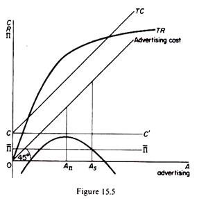
The sales maximiser will normally have higher advertising expenditures than a profit maximiser. In any case advertising cannot be less in a sales-maximising model. Baumol’s single-product model with advertising is shown in figure 15.5. Advertising outlay is measured on the horizontal axis and the advertising function is shown as a 45 line. Costs, total revenue and profits are measured on the vertical axis. Production costs are shown as being independent of the level of advertising (curve CC’). If these costs are added to the advertising cost line we obtain the total-cost curve (TC) as a function of advertising outlay. Subtracting the total cost from the total revenue at each level of output we obtain the total-profit curve Π.
The interrelationship between output and advertising and in particular the (assumed) positive marginal revenue of advertising permits us to see clearly that an unconstrained sales maximisation is (ordinarily) not possible. If price is such as to enable the firm to sell an output yielding profits above their minimum acceptable level, it will pay the firm to increase advertising and reach a higher level of sales revenue. The advertising outlay of the sales maximiser (0As) is higher than that of the profit maximiser (0AΠ), and the profit constraint (Π) is operative at equilibrium.
It should be stressed that the validity of this model rests on the crucial assumption that advertising always increases sales revenue. Baumol assumes that ∂R/∂a > 0, but does not establish the implied positive relation between total revenue and advertising. In particular Baumol does not examine explicitly the interrelationship between advertising, price, cost of production and level of output.
If total production costs are independent of advertising, (that is, production costs remain constant after advertising takes place) as Baumol assumes, this implies that total output X will remain constant after advertising has taken place; consequently an increase in sales revenue R, given X, can be attained only if P is raised. This case is in fact implied in figure 15.5, reproduced from Baumol’s book.
However, this is inconsistent with what Baumol states elsewhere (p. 60), that ‘unlike a price reduction a ceteris paribus rise in advertising expenditure involves no change in the market value of the item sold’. This statement implies clearly that advertising will not change the price. Hence Baumol implies that the increase in revenue will be attained from an increase in the volume X. But then production costs will increase, since MC is always positive.
In short, Baumol’s graphical representation of his model is inconsistent with his statements. In particular the price implications of a change in advertising are not obvious in Baumol’s analysis. Sandmeyer, Haveman and DeBartolo, and Kafoglis and Bushnell have highlighted this deficiency of Baumol’s model. They suggested that with advertising expenditures the TR curve will shift and in the new equilibrium revenue will be higher and advertising expenditure will be higher (consistent with Baumol).
However, output may be lower and price higher in the new equilibrium, depending on the shift and the elasticity of the demand curve following advertising, as well as on the cost conditions of the firm. This situation has not been explicitly envisaged by Baumol, whose model has been interpreted as implying that all ‘excess’ profit will be devoted to advertising and that, therefore, the increase in revenue will accrue from an increase in output resulting from the shift of the demand curve following advertising.
However, Baumol’s mathematical model allows for the possibility of a change in price as well as of advertising and output. Haveman and DeBartolo have presented a model which they call ‘generalized Baumol model’. In their model price, cost, output and advertising expenditure are all free to vary. We will first present graphically their model as modified by M. Kafoglis and R. Bushnell and by C. J. Hawkins. We will next present their model mathematically and will point out that actually their model is identical to Baumol’s mathematical presentation of his advertising model.
The cost curves. It is assumed that:
(a) Production costs vary proportionally with output. Thus the total production cost function is a straight (positively-sloping) line through the origin.
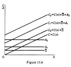
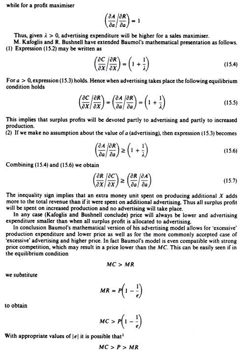
(b) Advertising expenditure may change but is independent of the level of output. Thus a given level of advertising is presented by a straight line parallel to the X-axis. Higher advertising levels are shown by parallel lines which are further away from the X-axis,
(c) The minimum profit constraint is exogenously determined and is denoted by a line parallel to the X-axis.
The total cost function is the summation of the production cost (C), the advertising expenditure (Ai) and the minimum profit constraint (Π). Given the production cost function and the minimum profit constraint, a change in advertising (Ai) will generate a family of total-cost curves which will be upward-sloping (with their slope equal to the slope of production cost function). Such a family of total-cost curves is shown in figure 15.6.
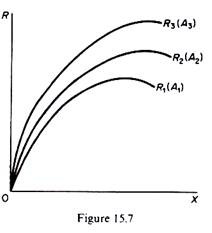
The revenue curves. The total-revenue curve has the usual shape, initially increasing but at a decreasing rate, reaching a maximum (where ∂R/∂X = 0), and then decreasing (as ∂R/∂X < 0). The total-revenue curve shifts upwards as advertising is increased. Thus, by changing advertising we may generate a family of total-revenue curves, each representing the relationship of total revenue to output at different levels of advertising expenditure. Such a family of total-revenue curves is shown in figure 15.7. Curve R1 is drawn on the assumption that advertising expenditure is Curve R2 implies an advertising expenditure of A2, and so on.
Equilibrium of the Firm:
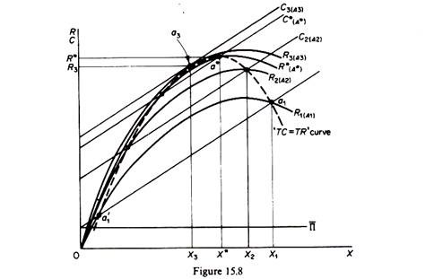
If we superimpose figures 15.6 and 15.7 and join the points of intersection of total-cost and total-revenue curves corresponding to the same amount of advertising expenditure, we obtain a curve which is called by Haveman and DeBartolo the TC = TR’ curve. It is the dotted curve in figure 15.8. The firm is in equilibrium when it reaches the highest point of this curve. The equilibrium of the firm is at point a*, with total costs C*, total revenue R*, output X*, advertising A*, and price equal to 0R*/0X*.
It should be clear that two conditions must be satisfied for equilibrium:
Firstly, the firm must operate on some point of the TC = TR’ curve. Secondly, MC > MR at equilibrium. Thus at point a., the first condition is fulfilled (C3 = R3) but the second condition is violated, since at a3 the two curves are tangent, implying MC = MR. Thus if the sales maximiser was producing at X3, he would substitute production expenditure for advertising expenditure (a reallocation of resources from advertising to increased production) until output increased to X*. In the process of adjustment price would fall, but the loss in revenue from this cause would be more than offset by the additional revenue from the increased output sold. In figure 15.8 we see that R* > R3.
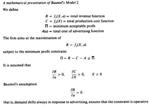
A mathematical presentation of Baumol’s Model 2
We define
R = ƒ1(X, a) = total revenue function
C = f2(X) = total production cost function
Π = minimum acceptable profit
A(a) = total cost of advertising function
Model 3: Multiproduct firm, without advertising:
If we assume that the firm has a given amount of resources (and given costs C) and wants to allocate them among the various commodities it produces so as to maximise sales revenue, it will reach the same equilibrium solution as the profit maximiser, that is, it will produce the same quantities of the various products as if it were a profit maximiser. Formally, the condition for the equilibrium of the multiproduct firm (with given resources and costs) is
which reads the firm is in equilibrium when the ratio of the marginal revenue from any two commodities (i and j) is equal to the ratio of their marginal costs.
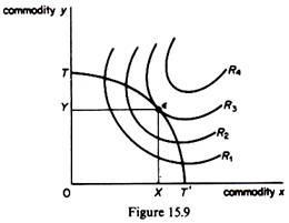
We may present the above solution graphically, assuming for simplicity that the firm produces two commodities, y and x. It involves the tools of the product transformation curve and of isorevenue curves.
The slope of the transformation curve is called the marginal rate of product transformation and is equal to the ratio of the marginal costs of the two commodities
The product transformation curve is concave to the origin showing the increasing difficulty (increasing cost) of reducing product y and reallocating the resources to the increase of product x.
An isorevenue curve shows the same revenue earned by different combinations of quantities of y and x. The further away from the origin, the higher the total revenue earned.
The isorevenue curve has a slope equal to the ratio of the marginal revenues of the two commodities:
The isorevenue curve is drawn convex to the origin, implying a falling demand curve for the two products, and hence a declining marginal revenue for additional units sold. (If prices were constant, the isorevenue curve would be a straight line with a negative slope, equal to the ratio of the prices of x and y.)
The firm is in equilibrium at point Ɛ where the given product transformation curve is tangent to the highest isorevenue curve. The firm maximises its sales revenue by selling 0X of commodity x and 0Y of commodity y.
This solution is identical with the equilibrium of a profit maximiser. There is nothing startling about this, since in both models we assume given resources and costs. The profit maximiser maximises
Π = R – C
Clearly, given C, whatever output combination maximises R also maximises profit Π.
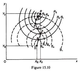
However, if the resources (and costs) are not given and the firm can allocate increased quantities of factors to the production of any product, the profit maximiser will have a different equilibrium product mix than the sales maximiser. This may be shown graphically by using isorevenue and isoprofit curves (figure 15.10).
The isorevenue curves have the same convex shape as previously. The isoprofit curves are concave to the origin, showing that the profitability of y and x decreases after a certain level of output, and may even become negative (losses) with a downward-falling demand curve for both commodities, revenues and profits decrease at high levels of output (as well as at low levels of output). Since the products compete for the resources of the firm, the closer to the origin an isoprofit curve is the higher the level of profit it depicts.
If the minimum profit constraint is Π1, the equilibrium of the sales maximiser is defined by point a on the isorevenue curve R6. Similarly, if the minimum acceptable profit is n2, the sales-maximising solution is b on curve R4. In general, the higher the profit constraint the lower is the attainable sales revenue.
Point R represents the unconstrained sales-maximisation solution; it is the level of sales where MR = 0, and is attained if the profit constraint is not operative, while point Π represents the profit-maximisation solution. Given the shapes of costs and demand curves implied by the isorevenue and the isoprofit curves, output levels of both y and x are higher for a sales maximiser than for a profit maximiser. In summary, if the resources (and costs) are not given, the multiproduct firm will reach a different product mix, depending on whether it is a profit maximiser or a sales maximiser.
The formal condition of equilibrium of a sales-maximising multiproduct firm may be stated as follows:
which reads the ratio of the marginal revenues of commodities i and j must be equal to the ratio of their marginal profitabilities. That is, the equilibrium of a sales maximiser is defined by a point of tangency of the isorevenue and the isoprofit curves; it will be a point on the curve Rabcde.
Model 4: Multiproduct model, with advertising:
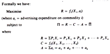
We will develop this model using calculus so as to achieve maximum generality. The firm aims at sales revenue maximisation subject to a minimum profit constraint.
From the solution of this constrained maximisation problem we obtain the levels of output (Xis) and the levels of advertising (ais) that maximise sales revenue and earn the minimum acceptable profit. We subsequently substitute the XiS into the demand functions of the individual products (which are assumed known) and obtain the prices.
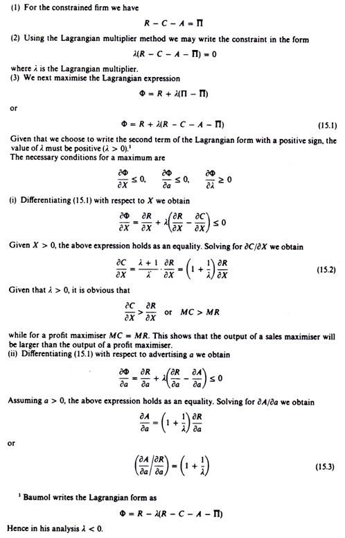
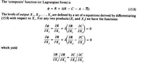
For the solution of the constrained maximisation problem we use the Lagrangian multiplier method.
This is the same condition as the one for model 3. Advertising does not alter this condition due to Baumol’s assumption that advertising is not a function of output.
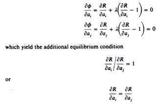
The levels of advertising expenses on each product, a1, a2, …, an are obtained from another
set of n equations derived by differentiating ɸ with respect to ai. Thus for any two products (Xi and Xj) we have
This condition states that the marginal revenue of advertising commodity i must be equal to the marginal revenue of advertising commodity j. If this were not so, the firm could increase R by reallocating the total advertising expenditure A among the different products, increasing advertising on those commodities for which the marginal revenue would be higher.
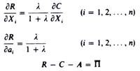
We thus have 2n + 1 equations to be solved for the n outputs (X1, X2, …, Xn), the n advertising expenditures (a1, a2,… ,an) and for the Lagrangian multiplier λ
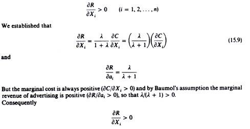
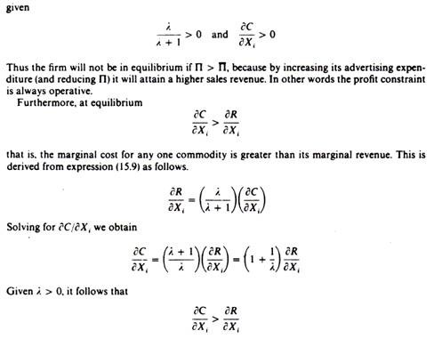
We may easily establish that with advertising included in the model the minimum profit constraint will always be operative. That is, the firm will not reach point R on figure 15.10, because it will be stopped at a lower revenue by the profit constraint. To prove this it suffices to show that the marginal revenues of the products are positive at the equilibrium solution, that is
This model can be extended to cover simultaneous changes in advertising and in output when surplus profits are earned.
IV. Baumol’s Dynamic Model:
The static single-period model developed in the previous section is only an introduction to the more ambitious multi period analysis attempted by Baumol. The most serious weakness of the static model is the short time-horizon of the firm and the treatment of the profit constraint as an exogenously determined magnitude. In the dynamic model the time-horizon is extended and the profit constraint is endogenously determined.
The Assumptions of the Dynamic Model:
1. The firm attempts to maximize the rate of growth of sales over its lifetime.
2. Profit is the main means of financing growth of sales, and as such is an instrumental variable whose value is endogenously determined.
3. Demand and costs have the traditional shape: demand is downward-falling and costs are U-shaped.
Profit is not a constraint (as in the static model) but an instrumental variable, a means whereby the top management will achieve its goal of a maximum rate of growth of sales.
Growth may be financed by internal and external sources. However, there are limits to the external sources of finance. Thus profits will be the main source for financing the rate of growth of sales revenue. For simplicity we may actually assume that growth will be entirely financed by profits.
The Multi period Model:
We assume that the sales revenue (R) grows at a rate of growth (g) per cent. Over its lifetime the firm will have a stream of revenues
R, R (1 + g), R (1 + g)2, … R (1 + g)n
The present value of this stream of future revenues is estimated by the usual discount formula
where i is the subjective rate of discount of the firm. The latter is exogenously given by the expectations and risk-preferences of the firm, and is higher than any form of market interest rate because it includes subjective assessment of risk.
The total present (discounted) value of all future revenues is
The firm attempts to maximise the present value of the stream of sales revenue over its lifetime, by choosing appropriate values for the current (initial) level of sales revenue (R) and its growth rate (g). It is obvious that S is positively related to both R and g: the present value of the stream of revenues will be higher for higher R and g values. Thus the firm should choose as large as possible values of R and g.
Given that g is financed (mainly or totally) by the internal profits one might ask whether sales maximisation makes sense as the goal of the firm in a multi period analysis. Surely by maximizing profits the firm could finance a higher rate of growth. Why then sacrifice current profits in favour of increased current sales? The answer to this question lies in the nature of the relationship between profits (Π), current sales (R), and the rate of growth (g). The growth function is
g= fi(Π, r)
where R, the current sales revenue, is an instrumental variable, and profits n are defined by the function
Π =f2(R, g, i, c)
(where C denotes costs).
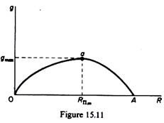
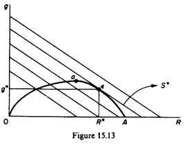
The growth function is actually derived from the profit function and is shown in figure 15.11. Expansion of the firm will depend on the current level of profits, because the retained portion of Π is the (primary) source of growth. Consequently the highest attainable growth rate (g) will be at the point of maximum profits. Beyond the level of sales revenue where profits are maximised, that is, beyond RΠm in figure 15.11, the growth rate will decline, as profits are declining.
In other words, up to point a, which corresponds to the maximum profit level, both the current sales revenue R and its rate of growth g increase simultaneously. Beyond that point, however, current sales revenue continues to increase but the rate of growth declines. Thus beyond RΠm sales revenue and growth become competing goals the firm has to choose between higher current revenue growing at a lower growth rate over time, and lower current sales growing faster over time. Clearly there is an infinite combination of values of g and R that the firm may choose. Among all possible values the firm will choose the pair of values of g and R that maximise the present value of the future stream of sales S.
To find the equilibrium of the firm we need an additional tool, the iso-present-value curve. This curve shows all combinations of g and R that yield the same S. Recall that from the definition of S
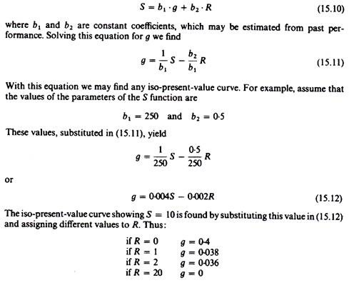
that is, the discounted value of the stream of future revenues is positively related to both g and R and negatively related to the subjective discount rate i. Given i (which is exogenously determined), the simplest relationship that can be postulated between these variables is of a linear form
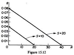
Plotting these pairs of g, R values on a graph and joining them with a straight line we obtain the iso-present-value curve S = 10 (see figure 15.12). By assigning different values to S and repeating the above process we may obtain a set of S curves. Under our assumptions the iso-present-value curves will be downward-sloping and will be parallel to one another.
Their slope is given by the ratio of the coefficients b, and b2 of the S function (that is, slope of S = b2/b1). Of course the S curves may be non-linear, of any form. The only requirement is that they have a negative slope, and this has been established on a priori grounds. Clearly the further away from the origin an iso-present-value curve lies, the higher the discounted stream of revenues it depicts.
The firm will choose the highest possible of the iso-present-value curves. That is, the firm is in equilibrium at the point of tangency of the growth curve (0aA) to the highest S curve (point Ɛ in figure 15.13). The point of tangency defines the equilibrium values g* and R*, that is, the attainable rate of growth and the level of current sales which maximizes the present value of the stream of future revenues (S* in figure 15.13).
The curve 0aA depicts the attainable growth rate (g) for any given value of current sales revenue (R). Growth is financed out of current profits, and the growth curve is therefore derived from the profit curve (On in figure 15.14). Note that at the origin and at the output level OB total profit is zero and hence the rate of growth is zero).
Given R*, we may determine the equilibrium level of output from the total revenue curve in figure 15.14. The sales maximiser will produce output X* and will sell it at a price equal to 0R*/0X*. Given the equilibrium output X* and the profit function, the profit constraint is now endogenously determined at Π *. In other words, the sales maximiser will require a profit level of Π * in order to finance the optimal growth rate g*.
The multi period model can be modified to allow for an exogenously determined minimum acceptable level of profit, as well as to allow for advertising and other non-price competition activities and for multiproduct activities.
The predictions of the multi period model are the same as those of the single-period model:
Output will be higher and price lower for a sales maximiser than for a profit maximiser if advertising is ignored. However, with advertising taking place there may be conditions under which these predictions will be different. (See the Haveman-DeBartolo version of the sales-maximisation model.)
Advertising expenditures will be higher for a sales maximiser, due to the assumption of a monotonic positive relation between sales revenue (r) and advertising expenditure.
An increase in overhead costs will lead to a reduction in output and an increase in price.
The levying of a lump-sum tax will have similar results: an increase in price and a reduction in output. The welfare implications of the behaviour of a sales maximiser are obvious. If the government imposes a lump-sum tax with the aim of redistributing income away from the taxed firm, its goal will not be attained, since the sales maximiser will shift the burden to his customers by charging increased prices.
Imposition of a specific tax will lead the sales maximiser to a larger reduction in output and a larger increase in price as compared with a profit maximiser. A shift in market demand to the right will lead to an increase in output and an increase in advertising, while the effect on p is not certain in Baumol’s model. However, in the Haveman-DeBartolo generalized model this prediction may not be true.
An increase in variable costs will lead the sales maximiser to an increase in price and a reduction in output. These changes will be greater than those of a profit maximiser.
V. Empirical Evidence:
Baumol claims that an increase in overheads, or the imposition of a lump-tax, both lead to an increase in the price charged by firms. This business practice, Baumol argues, provides evidence in support of his theory. However, the same business behaviour would be appropriate for a firm which sets its price at such a level as to prevent entry. Recall that according to all versions of limit-pricing, a general increase in costs, or the imposition of a tax that affects all firms in the industry in the same way, will induce firms to increase their prices, because they know that everyone will follow the same policy and thus there is no danger of losing market share.
In general the behavioural differences between long-run profit maximisation and sales maximisation are so subtle that no conclusive econometric tests can be carried out with the available data, most of which are compatible with various behavioural hypotheses. Sales maximisation is incompatible with an elasticity of demand of less than unity. Thus one would think that if the estimation of firms’ demand functions show ׀e׀ < 1, this would provide evidence against the sales-maximisation hypothesis. Yet there are so many variables that affect demand over time that econometric studies of individual demand functions become extremely tedious and mostly unreliable. No one has as yet published satisfactory results on individual demand functions.
McGuire, Chiu and Elbing attempted to test Baumol’s contention that ‘executive salaries appear to be far more closely correlated with the scale of operations of the firm than with profitability’. They chose 45 of the largest 100 industrial corporations in the United States and computed simple correlation coefficients between executive incomes and sales revenue (ryR) and profits (ryΠ) over the seven-year period 1953-59. Their results suggest that the correlation between executive incomes and sales revenue is stronger than the correlation between executive incomes and profits.
However, the authors recognise the serious limitations of simple correlation analysis, and in particular the fact that correlation does not necessarily imply causation, and they thus accept that their evidence is far from conclusive.
A more comprehensive empirical study was made by M. Hall. He attempted to test the hypothesis implicit in Baumol’s theory that if profits above the minimum constraint are earned, ceteris paribus, firms pursue policies (for example, cut prices, and increase advertising and investment) in order to increase their sales revenue.
He applied regression analysis to a sample of the largest American corporations, which operate in markets which fulfill the conditions of the sales-maximisation model. For each industry Hall estimated a minimum profit constraint (equal to the five-year mean profit rates for firms in the industry) and he assumed that this is the same for all the firms of his sample belonging to that industry. Hall’s regression model is of the general form
ΔSij = ƒ(ΔPij, A DiJ, ΔAij, V1, V2)
where ∆Sij = change in sales of the ith firm in the jth industry.
ΔPij = deviation of the actual profit from the minimum profit constraint of the ith firm in the jth industry.
ΔDij = change in industry demand.
ΔAij = change in assets of the ith firm in the jth industry.
V1, V2 = dummy variables to account for other factors that are common across firms in a given industry.
On a priori grounds (that is, if firms were sales maximisers) Hall expected a strong positive relationship between sales revenue changes and the deviation of actual from the desired profit (that is, the estimated profit constraint), since a positive departure of actual profits from the minimum acceptable level would induce the firms to pursue policies which increase sales revenue. However, his measurements revealed insignificant correlations between these variables, thus providing evidence against Baumol’s sales maximisation hypothesis.
L. Waverman questioned the empirical findings of Hall on the following main grounds:
(a) The influence of exogenous variables, such as changes in demand and prices of factors, had not been adequately taken into account; (b) the estimate of the minimum profit constraint could be questioned on several grounds; (c) the estimation method used by Hall was not appropriate due to errors of measurement of the profits available. Hall in an answer to Waverman accepts that the main defect of his study lies in the method of estimation of the minimum profit constraint, but he points out that this was the best he could do with the available data. This weakness, however, is very important and Waverman seems justified in questioning the results of Hall’s study.
Marby and Siders computed correlation coefficients between sales and profits (adjusted for trend) over twelve years (1952-63) for 120 large American Corporations. They argue that zero or negative correlations between sales and profits would support Baumol’s hypothesis. Their findings showed positive significant correlations between sales revenue and profits. This result does not necessarily contradict the sales-maximisation hypothesis, since sales and profits are positively correlated in Baumol’s model up to the point of maximum profits.
The authors, recognising this fact, concentrated on ‘reliable’ data of twenty-five firms, which, they thought, had been operating at scales of output beyond the levels corresponding to maximum profit. However, even in these cases the correlations between profits and sales were mostly positive. This evidence was interpreted as refuting the sales-maximisation hypothesis.
D. R. Roberts using a cross-section sample of 77 American firms (for the period 1948-50) found that executive earnings are correlated with the size of sales but not with the level of profits. This result provides evidence supporting Baumol’s claim that managers have strong reasons to pursue the expansion of sales rather than increase profits.
In summary, we can say that although various studies have been conducted to test Baumol’s hypothesis, the empirical evidence is not conclusive in favour of or against the sales-maximisation hypothesis.
VI. Some Comments:
The sales-maximisation hypothesis cannot be tested against competing behavioural hypotheses unless the demand and cost functions of individual firms are measured. However, such data are not disclosed by firms to researchers, and are commonly unknown to the firms.
It has been argued that in the long run the sales-maximisation and the profit-maximisation hypotheses yield identical solutions; because profits attain their normal level in the long-run and the minimum profit constraint will coincide with the maximum attainable (‘normal’) level of profit. This argument cannot be accepted without any empirical evidence to support it.
The sales-maximisation theory does not show how equilibrium in an industry, in which all firms are sales maximisers, will be attained. The relationship between the firm and the industry is not established by Baumol.
Baumol’s hypothesis is based on the implicit assumption that the firm has market power, that is, it can have control on its price and expansion policies. The firm can take decisions without being affected by competitors’ reactions.
Thus Baumol rules out interdependence ex hypothesi, and hence his theory cannot explain the core problem of uncertainty in non-collusive oligopoly markets.
The theory cannot explain observed market situations in which price is kept for considerable time periods in the range of inelastic demand.
The theory ignores not only actual competition, but also the threat of potential competition. It fails to see that if a firm encroaches on the share of firms in the same industry or other industries, reactions are bound to set limits to its discretion in expanding sales.
The assumption that the MR of advertising is positive (∂R/∂a > 0) is not justified by Baumol. And casual observation shows that this may not be so.
M. H. Peston ventured the idea that sales maximisation is not incompatible with the goal of long-run profit maximisation. A firm, he argues, may be willing to keep sales at a high level, even though they are unprofitable in the short run, in the hope that eventually (in the long run) the product will become profitable once established in the market.
Such behaviour is common for new products, for which the firm expects no profits or even losses at the initial stage of their introduction. However, firms expect to earn profits once their product becomes known in the market and captures a share at least equal to the minimum optimum scale. This behaviour, however, does not by itself provide a proof that the firm is a sales maximiser or a profit maximiser. After all, in Baumol’s model, sales and profits are not competing goals up to the level of output at which profit is maximised. Thus Peston’s argument does not seem to invalidate Baumol’s theory.
Peston also argued that firms may increase their sales beyond the level at which profit is maximised from sheer ignorance of their demand curve. If the LRAC is falling and firms miscalculate their demand, they almost certainly surpass the profit-maximising output.
Thus, Peston concludes, if firms are observed to sell too large an output, this does not show their preference for sales over profits, but may well be attributed to ignorance of demand conditions and the eagerness of firms to exploit technological changes which reduce costs at higher scales of output. We think that this argument of Peston’s does not contradict the sales-revenue-maximisation hypothesis. Even with falling costs the two goals are complementary over some scales of output but become competing beyond a certain level of output.
J. R. Wildsmith attacks Baumol on ‘intuitive’ grounds. He argues that the sales- maximisation model has the unacceptable implication that whenever profits above the minimum required level are earned ‘managers would derive extra satisfaction from huge outlays on advertising which brought negligible increases in sales and large reductions in profits’. Put in this way the argument seems plausible enough.
However, Wildsmith seems to overlook Baumol’s statement that although in his model only advertising is explicitly introduced for simplicity, other activities (such as change in the style of the product, increase of staff, increase of perquisites of managers, research and development expenses) may be incorporated in it without altering its basic mechanics.
Such activities are often undertaken (as well as additional advertising) when profits above the minimum required level are earned, and presumably they increase the utility of managers. Furthermore the ‘generalised Baumol model’ allows increases of output as well as increases in advertising when surplus profits are earned (see above, p. 333). Thus Wildsmith’s argument does not seem valid.
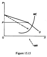
Shepherd has suggested that if the demand curve has a steep kink, so that to the right of the kink the MR is negative (figure 15.15), the goals of profit maximisation and sales maximisation would not be competing as Baumol implies, because under these conditions the firm’s equilibrium would be at the point of the kink. In other words, the ‘kinky’ solution would be chosen both by a profit maximiser and a sales maximiser.
This is easy to understand if we consider that the necessary condition of equilibrium for both types of firms is (provided that the profit constraint is operative). Since at the output corresponding to the kink MR > 0, while at any larger output MR < 0, it is clear that irrespective of goal (profit maximisation or sales maximisation) the firm will choose to produce the output corresponding to the kink.
∂R /∂X > 0
This argument has been attacked by Hawkins, who argues that Shepherd would be right if price were the only competitive weapon of firms. Given that in the modern oligopolistic industrial world advertising and other non-price weapons (for example, product changes) are the main instruments of competition, Shepherd’s argument is not valid.
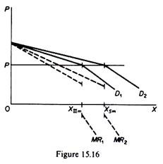
With advertising taking place the kinked-demand curve of a profit maximiser will be closer to the origin than the kinked curve of a sales maximiser, because the latter indulges in heavier advertising expenditures.
Thus both types of firms will operate at the kink of their demand curves (if beyond the kink MR < 0), but the output of the profit maximiser will be smaller than the output of the sales maximiser, because (at the same price level) the kink of the latter’s demand will occur to the right of the kink of the profit maximiser. This situation is shown in figure 15.16, from which it is obvious that Xnm < XSm at the same price, P.
Hawkins suggests that if in fact there is a steep kink in the demand curve Baumol’s model is improved, because its predictions (in case of shifts in the demand) become precise. With an accentuated kink, if demand shifts, advertising and output will increase, while price will remain unchanged, ceteris paribus, at the level of the kink.
Baumol claims that because in his model output will be larger than the output of a profit maximiser, the sales-maximisation hypothesis implies a lower degree of misallocation of resources and hence an increase in the welfare of the society. This claim is not necessarily true. The whole argument rests on the shape of the demand and cost curves as well as on the way by which one measures the society’s optimal output.
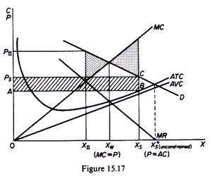
Assume that the cost and revenue curves are as shown in figure 15.17.
A profit maximiser will produce (at MC — MR) output XΠ and charge the price PΠ.
An unconstrained sales maximiser would produce X*s (where MR = 0). If he is constrained to have a maximum profit equal (say,) to the shaded area PSCBA, the sales maximiser will produce Xs and sell it at Ps.
Clearly Xs > XΠ and P, < PΠ. Profits also will be higher for the profit maximiser.
The question is: will the society be better off with a sales maximiser?
If the optimal output for the society is Xw (defined by P — MC), the sales maximiser’s output under the above conditions will be further away from the optimum output than the profit maximiser’s output. In this case the misallocation of resources (if measured as a departure of P from MC) will be greater for the sales maximiser.
However, if the society’s optimum is X* (where P = ATC inclusive of a normal profit), then the sales maximiser is preferable to a profit maximiser.
Thus Baumol’s claim, that his solution is preferable from the society’s welfare point of view, is not necessarily valid.
