Engineering costs are derived from engineering production functions.
Each productive method is divided into sub-activities corresponding to the various physical-technical phases of production for the particular commodity.
For each phase the quantities of factors of production are estimated and finally the cost of each phase is calculated on the basis of the prevailing factor prices.
The total cost of the particular method of production is the sum of the costs of its different phases.
ADVERTISEMENTS:
Such calculations are done for all available plant sizes. Production isoquants are subsequently estimated, and from them, given the factor prices, the short-run and the long-run cost functions may be derived. It should be noted that engineering production functions and the cost functions derived from them refer usually to the production costs and do not include the administrative costs for the operation of any given plant.
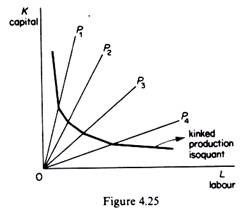
Engineering production functions are characterized by a limited number of methods of production. The production isoquants are kinked, reflecting the fact that factor substitutability is not continuous, but limited. Substitution of factors occurs directly at the kinks of the isoquants, where one production technique is substituted for another (figure 4.25). On the straight segments of the production isoquant a combination of the adjacent methods of production is employed. What happens in engineering production functions along the segments of the isoquants is an indirect substitution of factors via substitution of processes.
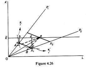
Assume that there are two methods of production, P1 and P2, using labour and capital at a fixed ratio, denoted by the slopes of the rays representing the two processes (figure 4.26). Assume that the factor prices are w and r, so that P1 is chosen initially and output X1 is produced, with ab of capital unemployed. The firm will be better off by using a combination of the two methods.
Thus at point e (where K intersects the higher isoquant X2) all K is employed. P1 and P2 are used at the levels 0A and 0B respectively, these levels being determined by drawing parallel lines to P1 and P2 through e.’ A substitution of factors has become indirectly possible (the K/L is defined by the slope of 0e), although K is given and the available technology does not allow substitution of K and L except by change of technique.
What happens at e is a substitution of processes instead of using P1 or P2 alone to produce X2, we achieve the same result (X2) by using a combination of Px and P2. Actually, given K and given the price ratio w/r, the output X2 is technically impossible to produce by using only P1 while X2 is not economically profitable to produce by using only P2 (given w/r), although with this process the level X2 is technically possible, since K does not limit effectively the production of X2, when P2 is employed. We turn now to the shape of total- and unit-cost curves when there are only a few processes available. The assumptions are that the prices of factors are given and the technology gives rise to kinked isoquants.
A. short-run engineering costs:
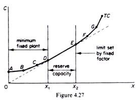
It is assumed that there is a fixed factor of production which requires a minimum outlay, and that there is some reserve capacity in the plant. The total-cost curve under these assumptions will be as in figure 4.27.
For the range 0X1 the TC is formed from linear segments, with the slope of each segment constant, but increasing for successive segments. The ends of linear segments correspond to outputs at which one process is replaced by another.
ADVERTISEMENTS:
(a) Along each linear segment the slope is the MC. Along the first segment (AB) the MC = A VC. For each successive section (that is, for sections BC and CD) the MC > A VC. The marginal cost increases step-wise while the AVC increases smoothly, at a decreasing rate.
(b) The AC falls continuously over the range ABCD. We said that the AC is the slope of the rays from the origin to any point on the TC curve. The slope of such rays declines as we move from A to B to C to D (figure 4.27).
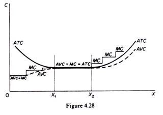
Over the range of reserve capacity the slope of total cost is constant. Furthermore this segment of TC lies on a line through the origin, reflecting the fact that only the TVC varies in proportion to output, while the fixed outlay has already been paid at the installation of the plant. The reserve capacity built into the plant allows the firm to operate by increasing only its variable costs proportionally with output. Thus over the reserve capacity segment the AVC, the MC and the ATC are equal and remain constant (between X1 and X2 in figure 4.28).
Once all reserve capacity is exhausted, output can be increased by overworking of the plant and paying overtime labour. The total-cost curve consists of linear segments, with each segment having a steeper slope than the previous one. Along each linear segment marginal cost is constant, but the level of marginal cost increases step-wise. The AVC increases continuously, but is lower than the MC. The average total cost increases continuously and lies below the MC but above the AVC. The short-run engineering-cost curves are shown in figure 4.28.
B. long-run engineering costs:
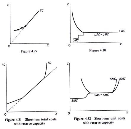
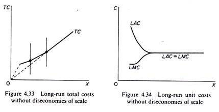
We said that the engineering costs include generally only the technical cost of production. Thus diseconomies of large scale, which are associated with administration costs, are not encountered here. There is a minimum optimal size of plant for each production process. The TC, AC and MC are shown in figures 4.29 and 4.30. If we assume that there is a very large number of processes, the total and unit cost curves become continuous (smooth) but retain broadly the above shapes, provided that there is a minimum fixed outlay and some reserve capacity in the short run (figures 4.31 and 4.32). In the long run the LAC will not turn upwards if we are considering only production costs; but if we add the administrative costs and if there are strong managerial diseconomies, the LAC will rise at very large scales of output (figures 4.33 and 4.34).
