As propensity to consume refers to willingness to consume so does propensity to save refers to willingness to save.
Saving is the difference between income and planned consumption, i.e.,
S = Y-C
Saving function is derived from the consumption function. Planned saving is a function of aggregate income, i.e.,
ADVERTISEMENTS:
S = f(Y)
Keynes’ saving function has the following characteristics:
1. Saving is a stable function of income.
2. Saving varies directly with income.
ADVERTISEMENTS:
3. The rate of increase in saving is less than the rate of increase in income. At very low levels of income as well as at zero income, since consumption is positive, saving must be negative. As income increases, dissaving vanishes and saving becomes positive. In Keynes’ terminology, this feature suggests that the value of the marginal propensity to save (MPS) is positive but less than one.
1. APS and MPS:
Before describing the Keynesian saving function, it is better to equip ourselves with the concepts of average propensity to save (APS) and MPS.
The complementary concepts of APC and MPC are APS and MPS, respectively. APS is the proportion of income devoted to savings. It is obtained by dividing total saving by total income, i.e.,
Table 3.1 suggests that when consumption exceeds income there occurs negative saving, so is the value of APS. When income and consumption are equal, APS becomes zero. Now, if income increases, APS would tend to rise.
ADVERTISEMENTS:
MPS is the change in saving consequent upon a change in income. It is the proportion of any addition to income that is used for saving. Symbolically,
MPS = ∆S /∆Y
The value of MPS is always less than one. In Table 3.1, MPS has been assumed to be 0.25, 1 i.e. 1/4. This means that an increase in national 4 income of Rs. 4 will lead to an increase in saving by one rupee. Here MPS is constant at all levels of income.
2. Saving Equation:
As consumption function equation is a linear one, so saving function must be a linear one:
S = Y – C = Y – (a + bY) [... C = a + bY]
or S = – a + (1 – b)Y [0< (l-b) < l]
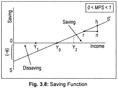
This is the saving equation in a linear form, a’ indicates negative saving represented by the vertical (negative) intercept as shown in Fig. 3.8. In terms of this figure, we find that saving function SS’ starts from the negative quadrant. Here (1 – b) is the MPS. If we know MPC (i.e., b) we can obtain MPS (i.e., 1 – b).
3. Saving Function in Graphic Form:
Fig. 3.8 depicts a linear saving function SS’. This function is a rising saving function. To indicate negative saving at zero level of income (i.e., negative saving represented by [- al), saving function starts to rise from the vertical axis below the origin. Now, as income rises, saving rises and, therefore, dissaving declines. At OY0 level of income, (since income equals consumption) saving is zero. That is why saving line at that level of income cuts the horizontal axis. To the left of OY0 level of income, as saving is negative, SS’ line lies below the horizontal line. To the right of OY0 level of income, as saving is positive, SS’ line lies above the horizontal line.
The slope of the saving function is given by the MPS. To calculate MPS, we have chosen two points ‘r’ and ‘h’ on the line SS’. As we move from ‘r’ to ‘h’, national income (A Y) rises by rn amount and saving (AS) rises by nh amount. Thus,
MPS = ∆S/∆Y = nh/rn slope of the SS’ line.
The value of MPS is always positive but less than one.

