In this section we will extend the analysis to the multiproduct firm. We simplify the exposition by assuming that the firm produces two products, X and Y.
The analysis can easily be extended to any number of products.
A. The Production-Possibility Curve of the Firm:
Each product is assumed to be produced by two factors, L and K. For each product we have a production function
ADVERTISEMENTS:
x = f1(L, K)
y = f2(L, K)
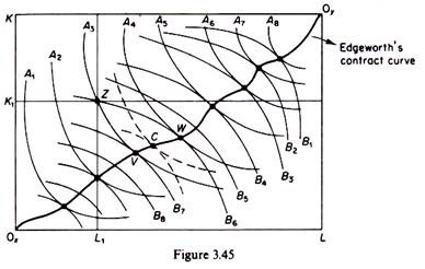
Each production function may be presented by a set of isoquants with the usual properties. We may now obtain the production-possibility curve of the firm by using the device of the Edge-worth box. We assume that the firm has total quantities of factors 0L and 0K (figure 3.45) measured along the sides of the Edge-worth box. Any point of the Edge- worth box shows a certain combination of quantities of x and y produced by the available factors of production.
The production function for commodity x is represented by the set of isoquants denoted by A which are convex to the origin 0X. The production function for commodity y is represented by the set of isoquants denoted by B which are convex to the origin 0y. The further down an isoquant B lies, the higher the quantity of y it represents. The two sets of isoquants have points of tangency, which form the contract curve.
ADVERTISEMENTS:
Only points lying on the contract curve are efficient, in the sense that any other point shows the use of all resources for producing a combination of outputs which includes less quantity of at least one commodity. For example, assume that initially the firm produces at point Z, at which the quantity of x is A3 and the quantity of y is B6. The production of the level A3 of x absorbs 0xL1 of labour and 0XK1 of capital. The remaining resources, L1L and K1K, are used in the production of commodity y.
It can be shown that the firm can produce more of either x or y or of both commodities by reallocating its resources so as to move to any point between V and W on the contract curve. If the firm moves to W it will be producing the same level of y(B6), but a higher level of x(A4). If the firm chooses to produce at V, it will produce the same quantity of x(/l3), but more of y(B7).
Finally, if the firm produces at any intermediate point between V and W, for example at point C, it will attain higher levels of production of both x and y. Thus points on the contract curve are efficient in that any other point off this curve implies a smaller level of output of at least one product. The choice of the actual point on the contract curve depends on the ratio of the prices of the two commodities (see below).
ADVERTISEMENTS:
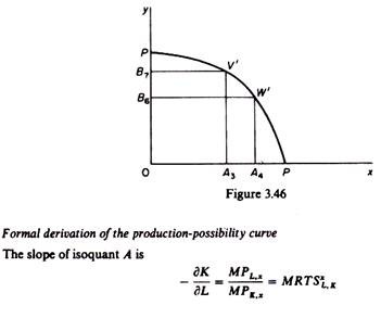
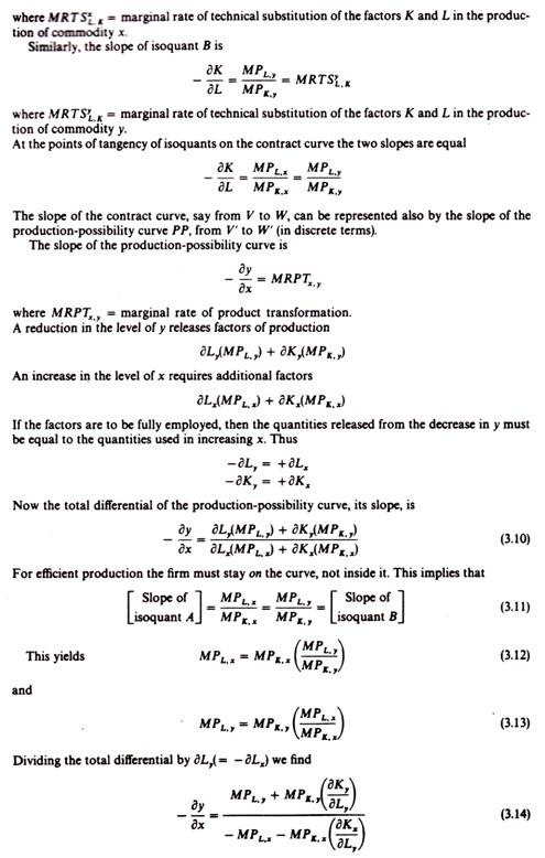
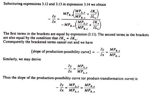
To determine the choice of levels of x and y we need to derive the production-possibility curve (or product-transformation curve) of the firm. This shows the locus of points of levels of x and y which use up all the available resources of the firm. The production- possibility curve is derived from the contract curve. Each point of tangency between isoquants, that is, any one point of the contract curve, defines a combination of x and y levels of output which lies on the production-possibility curve. For example, point V, representing the output pair A3 from x and B7 from y, is point V on figure 3.46. Similarly point W of the contract curve is point W’ on the production-possibility curve.
The optimal combination of the output pair is the one which yields the highest revenue, given the production-possibility curve, that is, given the total quantities of factors which define this curve. To find the equilibrium of the firm we need an additional tool, the iso-revenue curve.
B. The Iso-revenue Curve of the Multiproduct Firm:
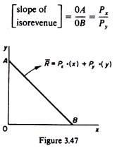
An iso-revenue curve is the locus of points of various combinations of quantities of y and x whose sale yields the same revenue to the firm (figure 3.47).
The slope of the iso-revenue curve is equal to the ratio of the prices of the commodities:
Proof:
ADVERTISEMENTS:
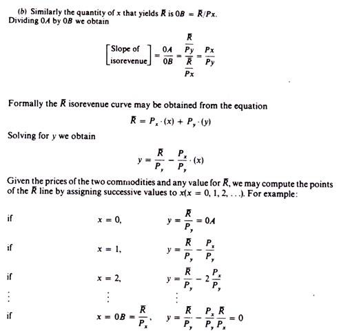
Assume that we want an iso-revenue depicting R total revenue.
(a) If we sell only y the total revenue is (0A). Py = R, that is, the quantity of y which yields R is (0A) = R/Py.
ADVERTISEMENTS:
We may in the same way define the whole set of isorevenue curves by assigning to R various values. The further away from the origin an isorevenue curve is, the larger the revenue of the firm will be.
C. Equilibrium of the Multiproduct Firm:
The firm wants to maximize its profit given:
ADVERTISEMENTS:
(i) The constraint set by the factors of production,
(ii) The transformation curve, and
(iii) The prices of the commodities (Px, Py) and of the factors of production (w, r).
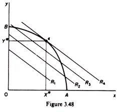
Assuming that the quantity of the factors and their prices are given, then maximization of n is achieved by maximizing the revenue, R. Graphically the equilibrium of the firm is defined by the point of tangency of the given product-transformation curve and the highest iso-revenue curve (figure 3.48). At the point of tangency the slopes of the iso-revenue and the product-transformation curves are equal.
Thus the condition for equilibrium is that these slopes be equal:
