The Production Process (With Diagram)

In this article we will discuss about the Theoretically Analysis of the Production Process.

Production Process:

The business firm is basically a producing unit it is a technical unit in which inputs are converted into output for sale to consumers, other firms and various government departments.

Production is a process in which economic resources or inputs (com­posed of natural resources like land, labour and cap­ital equipment) are combined by entrepreneurs to create economic goods and services (also referred to as outputs or products).

Inputs are the beginning of the production process and output is the end of the process. Fig. 13.1 is a simple schematic presentation of the production process, which can be conceived of as transforming inputs into outputs.

It is to be noted at the outset that the process may produce as joint products both goods and services (which are desired by consumers) and commodities such as pol­lution (which is not desired by consumers).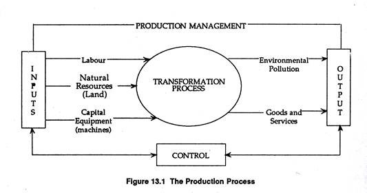

In traditional economics, the term ‘production’ is used in a broad sense. It refers to the provision of goods and services for sale in the market with a view to satisfying human needs and wants.

In man­agerial economics, however, the term is used in a narrow sense to refer to the processes of physical transformation of resources, such as the transforma­tion of iron ore into steel or the production and as­sembly of components into a finished car.

This defi­nition surely includes other and equally vital forms of transformation such as that of location, whereby the finished car is moved from the factory to the showroom of the dealer from whom it can be pur­chased. Here we concerned with production in the narrow sense of physical trans­formation, with particular reference to economic problems connected with production in the factory.

The production system can be seen as consisting of three elements – inputs, the production process and outputs. In reality, the outputs are the start­ing point of the operation inasmuch as they must be considered in the light of the market possibili­ties.

Inputs take the form of labour of all types, the required raw materials and sources of energy. All these involve cost outlays. Thus the theory of cost and theory of production are interrelated. In fact, the former is derived from the latter.

The production system can be shown as a con­tinuous, smooth flow of resources through the pro­cess ending in an outflow of a homogeneous product or two or more products (in fixed or variable pro­portions).

Time also plays a very important role in the the­ory of production. We usually draw a distinction between the short run and the long-run. The distinc­tion is not based on any time period but is made on the basis of the possibility of factor substitution.

In the short run, it is assumed that some factors (such as capital or plant size) remain fixed and others are variable. In the long run, it is assumed that all fac­tors are variable. From this we drive the proposition that the short run costs are partly fixed and partly variable; in the long run all costs are variable.

Finally, in traditional economics it is assumed that the techniques of production are ‘given’. But in managerial economics, however, it is assumed that there are usually various alternatives open to the manager from which one has to be selected.

Production Decision:

The theory of production lies at the heart of managerial economics. It forms the foundation for the theory of supply, which, is one of the basic concepts in the deter­mination of prices. Furthermore, production deci­sions are an important part of managerial decision making.

Managers are required to make four different but interrelated production decisions:

(1) Whether or not to actually produce or to shut down;

(2) How much to produce;

(3) What input combination to use and

(4) What type of technology to use.

Simply put, production involves the transfor­mation of inputs – such as capital equipment, labour, and land – into output of goods or services. In this production process, the manager is concerned with efficiency – technical and economic – in the use of these inputs. And the efficiency goal pro­vides us with some basic rules about the manner in which firms should utilize inputs to produce desir­able goods and services.

In fact, the theory of production is just an ap­plication of the constrained optimization technique. The firm seeks either to minimize the cost of pro­ducing a given level of output or to maximize the output attainable with a given level of cost.

It will be evident that both optimization problems lead to the same rule for the allocation of inputs and the choice of technology. And this rule is applicable to variable resource allocation problems. We may ap­ply the rule in the discussion of input markets and input demand by a firm.

We start with a general discussion of what is meant by a production function. In fact, the key concept in the theory of production is the produc­tion function, which is a technical relation showing how inputs are converted into output.

It is also an economic relation indicating the maximum amount of output that can be obtained from a fixed amount of resources (inputs). The issue of joint and multiproduct firms will be treated separately. To start with, we shall consider production in the short run, when only one input is variable.

Next we shall consider production and the optimal combination of inputs when two or more of the inputs can be varied. We shall do some comparative statics exer­cises, i.e., we shall consider the effect of an increase in all inputs on total output and consider the effect of changes in factor prices on factor proportion or relative input usage.

The Production Function:

The production function is the key concept of production theory because it is the link between in­put usage and an attainable level of output. It for­mally describes the relation between physical rates of output and physical rates of input usage. With a given state of technology, the attainable level of output depends largely, but not entirely, upon the quantities of the various inputs employed in the pro­duction process.

A production function is usually defined as a schedule (or table, or mathematical equation) show­ing the maximum amount of output that can be produced from a fixed amount of resources, given the existing technology or the art of production. In short, the production function is a catalogue of a firm’s output possibilities.

Various inputs are normally used in production. So as a general rule, we can define maximum output, Q to be a function of the level of usage of the various inputs, X, that is,

Q = f (X₁X₂,…X_n).

But in our discussions we shall focus on the simpler case of one output produced using either one input (labour) or two inputs (capital and labour). Hence, the production function may be expressed as

Q = f (K, L).

However, the principles we will develop can be extended to cover situations involving more than two inputs.

We have noted earlier that the production func­tion shows the maximum amount of output that can be produced from specified levels of input usage. For example, suppose the production function indi­cates that by combining 10 units of capital with 40 units of labour (however measured) we can produce 100 units of output per period.

However, 10 units of capital and 40 units of labour could produce less than 100 units of output if they are used inefficiently, but they can produce no more. If we want more out­put we have to increase either labour or capital, or both.

i. Fixed and Variable Factors:

While analysing the process of production, eco­nomists find it convenient to classify inputs into two categories: fixed or variable. A fixed input is one whose level of usage cannot readily be changed. However, in practice no input is absolutely fixed for­ever, no matter how short the period of time un­der consideration.

However, while all inputs are in fact variable in practice, the cost of immediate variation in the use of a particular input is often so great that such an input is not varied. For example, buildings, major pieces of machinery, and manage­rial personnel are inputs that generally cannot be varied quickly.

Therefore, such variation is unlikely to affect short-term production decision. A variable input, on the other hand, is one whose level of us­age may be increased or decreased readily and con­tinuously in response to desired changes in output. Various types of labour services as well as certain raw and processed materials could be placed in this category.

On the basis of such classification of inputs, economists draw a distinction between the short run and the long-run. The former refers to that period of time in which the level of usage of one or more of the inputs is fixed. Therefore, in the short-run, output is basically a function of the quantum (us­age) of the variable factors, i.e., changes in output must be accomplished exclusively by changes in the use of the variable inputs.

Thus, more output can be produced in the short run by using more hours of labour (a variable service) and other variable inputs, with the existing plant and equipment (or the stock of capital). In a like manner, if producers wish to reduce output in the short run, they may reduce the quantum (usage) of only variable inputs.

A build­ing or a blast furnace cannot be discharged (even though its use may fall to zero). In any discussion of short run production function, capital is taken to be the fixed input. So output is a function of labour alone.

Such a simplified production function may be expressed as:

Q = ƒ(K̅, L), (1)

where the bar over capital means that it is fixed.

Alternatively, it can be expressed as:

Q = ƒ (L) (1).

By contrast, the long-run refers to the period of time (or planning horizon) in which all inputs are ca­pable of continuous variation. The long-run, in other words, refers to that time in the future when out­put changes can be accomplished in the most cost- effective manner.

For example, in the short run, a producer may be able to expand output by operating the existing plant more intensively. In the long-run, it may be more economical to create additional ca­pacity, i.e., productive facilities to produce any extra output that may be required to meet demand.

ii. The State of Technology or Applied Scientific Knowledge:

From the technological point of view, a produc­tion function is a still picture of the production pro­cess at a fixed point in time. This is, it is based on un­changed technology or art of production.

Thus, if a firm, say a computer manufacturer is utilizing the most up-to-date technology, and if this technology is modified, from say transistors to silicon chips, then the production process and the production function must undergo change accordingly.

It is so because in a competitive world the production managers will be compelled to use the technology that is most cost effective.In this context one may draw a distinction be­tween efficiency and effectiveness. While effective­ness means doing the right things efficiency refers to doing things right.

Thus, we observe that the production process is time-specific. Both inputs and outputs are expressed as flows per period of time. For example, produc­ing one computer every two hours is equivalent to suggesting that the process is producing at the rate of half a computer per hour. Because output is mea­sured per unit of time, inputs must also be measured in terms of services provided for each time period.

For instance, six hours of labour input and six hours of machine usage may mean six workers each using one machine for one hour (process A), or one worker using one machine for six hours (process B). The inputs are the same in each case, but for the produc­tion manager, it makes a lot of difference whether process A or B is selected and used.

iii. The Short-run Production Function with One Variable Input:

The most basic form of the short run production function was presented in Equation (1) or (1)’ and contains one variable input. We may now proceed a step further.

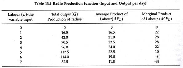
Let us suppose that we have collected necessary information on the relationship between the number of radios produced per month and the labour (L) utilized on a monthly basis as noted in Table 13.1.

The information in Table 13.1 was derived on the basis of the following production function for radios:

Q = 10L + 7.5L² – L³ (2)

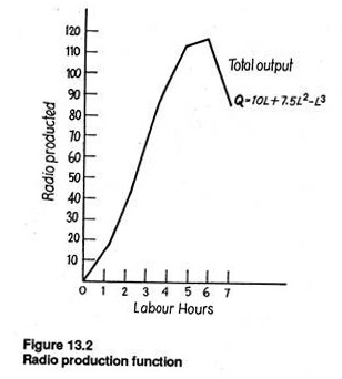
Here the radio production function as presented in Fig. 13.2 is 5-shaped. The production function is a short-run production function because it illustrates what happens to output as more and more units of the variable input, labour, are added to the fixed stock of capital.

Thus Fig. 13.2 is a graphic repre­sentation of equation (2) which is the short-run pro­duction function for radios. Table 13.1 and Fig. 13.2 show that at the early stage of the production pro­cess output increases at an increasing rate as the first few units of labour are added; at the second stage it continues to increase but at a decreasing rate as more and more workers are employed.

In Fig. 13.2 output reaches a maximum of approximately 114 ra­dios when six units of labour are combined with the fixed quantity of capital.

From the total product curve we can derive the average physical product or average product (AP) curve and the marginal physical product or marginal product (MP) curve. In the above example, both average product and the marginal product concepts refer to labour (L), the only variable factor of pro­duction.

Here we shall call total output by the name total product or total physical product. In a like manner the terms input, economic resource, or factor of pro­duction represented by L or K, is used to denote the resources used in the production process.

From the total product curve we derive the average phys­ical product or average product (AP) curve and the marginal physical product or marginal product (MP) curve. In the radio example, both average product and the marginal product concept refer to labour (L), the only variable factor of production.

iv. Average Product of Labour:

The average product (AP) is output per work­er. It can be defined as the total product divided by the quantity of the variable input (i.e., the num­ber of workers) employed.

In the case of the above production function, the average product of labour (AP_L) is expressed as:

By specifying different values of labour, we can determine the average product of labour at different levels of input usage, as illustrated in Table 13.1. If we are interested in finding out the level of labour usage that maximizes average product, we have to take the first derivative of equation (3), set it equal to zero, and solve as follows:

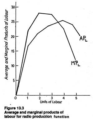
Thus, the average product of labour is maxi­mum at 3.75 units of labour. Fig. 13.3 graphically illustrates the behaviour of the average product of labour for the radio production function. The average product of the variable resource (labour) provides management with a measure of the efficiency of the input.

For example, in the case where no variable input is used, total output is zero. Thus positive quantities of the variable factor are to be used to get any output at all. It is because the fixed factor of production is being underutilized in the absence of labour.

The first unit of labour results in 16.5 radios being produced, and the second unit of labour (when combined with the first unit and the fixed resources) results in 42 radios being produced and so on. Thus, the average product for one unit of labour is 16.5 radios and for two units of labour 21 radios.

An important point to note in this context is that when two units of labour are employed, the aver­age product of labour increases. Thus two units of labour are clearly more efficient than one unit. This does not necessarily mean that the second unit of labour is more efficient than the first unit.

The in­crease in average labour productivity when the sec­ond unit of labour is employed in the production process is a result of a more efficient use of both the fixed factor of production and the first unit of labour. For example, it is quite possible that when the extra unit of labour is employed, the production process will become more specialized, thereby en­abling both workers to be more efficient or produc­tive.

This, too, has important practical implications for both the production manager, interested in set­ting up the flow of work, and the personnel man­ager, who designs pay scales. The second worker should not be paid more than the first, but both workers may develop the feeling that they should be rewarded because of higher per capita produc­tivity.

v. Marginal Product of Labour:

In economics, the word ‘margin’ always refers to anything extra. Thus, the marginal product of the variable factor (labour) may be defined as the rate of change in total output associated with the employment of one additional unit of the variable factor. To find out the marginal product we have to take the first derivative of the production function. In our radio production example, the marginal product of labour ( MP_L) can be computed as

Given the marginal product of labour function in Equation (5), the specific values associated with particular levels of labour input are noted in the fi­nal column of Table 13.1. Each of these values is obtained by substituting values of L into Equation (5) and solving for marginal product.

The informa­tion in this column is illustrated graphically in Fig. 13.3. The marginal product of labour is measured by the slope of the total product curve at a particu­lar point, dQ/dL .The slope of the total product curve is initially positive (implying positive MP_L), then zero (implying zero MP_L or constant total product) and ultimately negative (implying negative MP_L.)

Alternatively, the average marginal product or marginal product per unit of labour input can be calculated over an input range by simply relating the absolute change in output (∆Q) to the absolute change in the variable (factor) input (∆L). Thus when the second unit of labour is employed, MP_L per unit is 25.5 units:

Average M P_L = ∆Q/∆L = (42.0-16.5)/(2-1)= 25.5.(6)

Thus, over the range from one to two units of labour, average marginal product is 25.5 units. In our example, each unit of labour = 10 workers. Therefore, average MP_L = 255.5/10 = 2.55.

When L equals 2, however, the marginal product of labour (shown in Table 13.1) is 28 units (or aver­age MP_L = 2.8 units). This distinction between the marginal value at a single point on a curve, and the marginal value between the two points on a curve bears relevance in managerial decisions involving cost and output.

Properties of Production Functions:

We may now turn to the fundamental issue of the properties of the short run production function and the implications of these properties for practicing managers against this backdrop.

i. The Law of Diminishing Returns:

The shape of the total product, average product and marginal product curves depend largely on a fundamental technological law, viz., law of dimin­ishing returns originally discovered by two classical economists, viz., David Ricardo and T. R. Malthus.

The law is alternatively called the law of variable pro­portions or, because of the inverse relationship be­tween costs and productivity, and the law of increasing (marginal) op­portunity costs.

The law of diminishing returns sim­ply states that as the quantity of a variable input is increased by additional equal increments, while keeping all other factors and the state of technology unchanged, the increment to total output will even­tually decline.

In other words, as more and more unit6 of the variable factor are applied with a fixed quantity of other factors, every additional unit of the variable factor will gradually make less and less contribution to the total product.

Differently put, the contribution of the last worker to TP_L will gradu­ally diminish. It is because the variable factor will gradually have less and less units of the fixed factor to work with. The essence of the Law of Variable Proportions may be stated thus: If all the inputs can­not be varied proportionately in the short run, output will follow the Law of Non-proportional Returns.

The Law of Diminishing Returns holds in the short-run because all factors except one are kept un­changed. The only decision to be made by manage­ment in case of the radio production function was to determine the appropriate quantum of labour to be used in the production process.

Furthermore, the state of technology is also assumed to remain con­stant. Finally, the law of diminishing returns refer to the point at which the marginal product of the vari­able factor begins to decline, not the point at which it becomes negative (i.e., when total product itself falls).

The law of diminishing returns is an empirical law of production. It was first discovered from the experience of the farmers. It is, in reality, a state­ment concerning the physical relationship between different amounts of a variable input and the result­ing output.

The law is universally applicable. If the law did not hold in virtually all short-run produc­tion situations, production managers would never stop using additional units of a variable factor of production, because MP_L would always be posi­tive.

For the radio production function, the operation of law of diminishing returns starts when 2.5 units of labour are employed.

To verify this we have to take the first derivative of the marginal product of labour function, set it equal to zero, and solve for L to get:

Alternatively, the operation of the law or hy­pothesis of diminishing returns could easily be test­ed by simply taking the second derivative of the total output (product) function.

ii. The Total-Marginal Relationship:

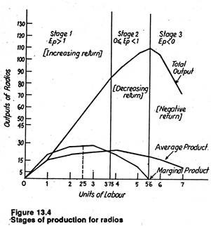
Fig. 13.4 presents the relationships among all three product curves as they are derived from the radio production function. Because the marginal product is measured by the slope of the total product curve, marginal product is equal to zero when the slope of the total product curve is zero (i.e., when total product reaches the maximum level).

This hap­pens when output is 115.6 units and labour input is 5.6 units. If more than 5.6 units of labour are used to­tal product will actually decline and marginal prod­uct will become negative.

The point at which diminishing returns set in, 2.5 units of the variable input labour, is also the point at which the slope of the total product curve be­gins to fall. In mathematics, this point is known as the point of inflexion, and it occurs when the second derivative of the total product curve equals zero.

The total product curve reflects the following assumptions:

1. No output can be produced with zero level of labour (this point has already been noted).

2. Output, first increases at an increasing rate. In Fig. 13.4 this occurs when 2 workers are employed. Over this range, marginal product is increasing.

3. Total product thereafter increases but at a decreasing rate, i.e., between 3 and 5.6. Over this range marginal product is diminishing.

4. Finally, a point will be reached beyond which total output itself will actually fall, indicating a neg­ative marginal product. In Fig. 13.4, this occurs for employment levels greater than 5.6.

iii. The Average-Marginal Relationship:

There is also a very close relation between MP_L and AP_L. The following three points are worth not­ing in this context:

1. So long as the marginal product curve lies above the average product curve, the average prod­uct curve will rise. The implication is that the aver­age efficiency of the variable factor is increasing.

2. Whenever marginal product is less than av­erage product, average product will diminish.

3. Thus, it logically follows that marginal prod­uct must be equal to average product when the latter reaches its maximum, i.e., when it is neither increas­ing nor falling.

This in our example occurs when 3.75 units of labour are used in the production pro­cess. That is, given the fixed amount of other factors of production, the maximum output per worker oc­curs when 3.75 units of labour are used. These three points may be proved mathematically.

It may be noted in passing that average product continues to increase even after the marginal prod­uct of the variable input has started declining. Aver­age product will continue to rise so long as marginal product is greater than average product.

The point at which average product reaches its maximum is the point of maximum production efficiency in the short run. However, this is not necessarily the point at which profits will be maximized. Market prices of the various factors must be brought into consider­ation with productivity data before factor costs can be clearly analysed.

Elasticity of Production:

The elasticity of production can be defined as the ratio of percentage change in output to the per­centage change in the amount of the variable input.

It measures the degree of responsiveness of total output to a small change in the variable input.

For continuous changes in L and Q, the elastic­ity of production can be expressed as

A close look at Equation (9) reveals that the elasticity of production is simply the ratio of the marginal product to the average product of the vari­able factor (labour), i.e.,

For the radio production function in Equation (2) the elasticity of production is, therefore, equal to

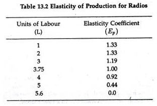
Table 13.2 furnishes details of the results of sub­stituting values for the variable input, labour, into Equation (11).

From Table 13.2 we discover the important re­sult that up to 3.75 units of labour (L), the elasticity of production exceeds 1, indicating that output is in­creasing faster than input usage. This itself is a test of the efficiency of the production process.

When 3.75 units of labour are combined with the fixed factors of production, the elasticity of production is equal to exactly 1, indicating that production is increasing at a rate at which labour usage is increas­ing. Whenever more than 3.75 units of labour are used, output is still increasing, but more slowly than labour usage.

Beyond 5.6 units of labour, output is actually falling despite the fact that the amount of labour usage is increasing. The labour input value of 3.75 units corresponds to the “peak” of the AP_L, curve, i.e., maximum AP_L, and is also a cut-off or critical point for elasticity of production.

The elasticity of production has greater practi­cal implications for production managers who are being asked to raise and lower output on a periodic basis. The concept makes it clear that 20% increase in output will not always necessitate a 20% increase in labour usage.

Three Stages of Production and Decision Making:

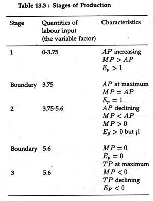
From our discussion so far we have discovered three different stages of the production process in the short-run. Each stage is important from the stand­point of efficient resource utilization (as shown in Fig. 13.4). All the three stages together constitute what is broadly called the Law of Variable Propor­tions.

In stage 1, marginal product exceeds average product. In our example, stage 1 starts when the amount of labour is equal to zero and continues up to the point where 3.75 units of labour are employed. In this initial stage the fixed factors of production are not pressed into service fully and maximum produc­tion efficiency is not achieved.

This is quite obvious that if no labour input is used, output will be zero, despite the fact that fixed factors of production are available. This is because the fixed factors of production cannot be utilized ef­ficiently without sufficient use of the labour input.

From the point of view of economic feasibility the relationships in stage 1 suggest that production should be continued until stage 2 has been reached. The implication is that the profit-oriented will not will surely seek to expand production all the way through stage 1.

This is because so long as aver­age product is increasing, the production process is becoming more and more efficient (increasing the number of radios produced per unit of labour).

This is the case throughout stage 1 in as much as the aver­age product of labour is a measure of its efficiency. Therefore, continuous increase in the use of the vari­able factor throughout stage 1 is warranted. In our example, the production decision maker should in­crease the use of labour up to at least 3.75 units.

In stage 3 total product is itself falling. Thus the rational decision maker will not use more than 5.6 units of labour, whatever be its price. Beyond this point every extra unit of labour will actually lead to a fall in total output.

Moreover, the elasticity of production is negative in stage 3, thus forcing the same conclusion. Stage 2 and its boundaries are the economically feasible region, i.e., the area within which the rational producer will choose to operate.

The exact amount of labour that should be used so as to maximize profits can be determined only after knowing the prices of inputs and outputs. However, it is known to us that the firm will use between 3.75 and 5.6 units of labour.

Table 13.3 summarizes the relationships that ex­ist in, each of the stages of production in the short run.

Production with Two or More Variable Inputs:

We may now extend our analysis to cover more than one variable input. The principles developed in this section will continue to apply. We may con­tinue to assume that at least one of the factors of production is fixed in quantity. This implies that we are still dealing with the short run, in which case the law of diminishing returns will apply.

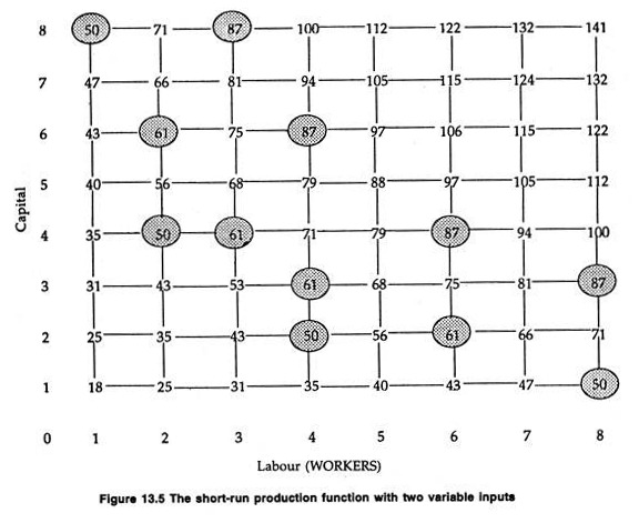
Capital inputs are measured vertically and labour inputs are measured horizontally (see Fig. 13.5). The number at the intersec­tion of a row and column shows the output for that level of capital and labour input.

For example, 4 machines and 2 workers produce 50 units of output. The operation of law of diminishing returns can also be discerned. When the input of machines is held constant at 4 units, then additional units of labour bring about smaller and smaller additions to output. Thus, along a given row output increases, but at a decreasing rate.

If all inputs are variable, the law of diminishing returns will not apply, and the short run is replaced by a long-run period in which case the decisions to be made by the firm are distinctly different.

Example:

Production managers of the Metal Box Co. esti­mate that their production process is currently char­acterised by the following short-run production function:

Q = 72X + 15X² – X³,

where Q = tonnes of boxes produced per production period and

X = units of variable input employed per production period.

(a) Graphically illustrate the production func­tion, indicating the following:

i) The range of increasing returns;

ii) The range of decreasing returns.

(b) Determine the equation for the MP and AP of the variable factor.

(c) What is the marginal product when seven units of the variable input are employed?

(d) What is the maximum output capability per period?

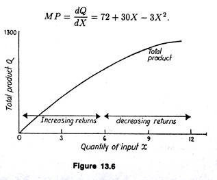
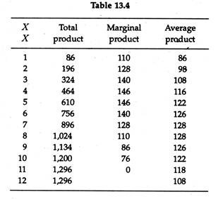
(a) The production function is Q = 72X + 15X² – X³ and from this equation for total prod­uct Q we can derive marginal and average product figures by putting in the equation, different values for X (See Table 13.1). Total product curve is shown in Fig. 13.16 below.

The law of decreasing returns starts to operate when the seventh man is employed, i.e., the output produced by each additional unit of the variable factor X after the sixth, begins to fall. Conversely, increasing returns apply up to and in­cluding the sixth unit of the variable factor.

(b) The marginal product of X represents the rate of change of the total product schedule.

Thus differentiating total product (TP) with respect of X gives us the MP equation:

The average product equation is simply derived by dividing the total product by the variable input X. Thus we get,

Ap = 72X + 15X² –X³/X =72+15X – X²

(c) To find out the marginal product when seven units of the variable input are employed, requires the substitution of the relevant number into the MP equation:

MP = 72 + 30 X 7 – 3 x 7² = 72 + 210 – 147 = 135.

(d) The maximum output capacity in the short term can be obtained in two alternative ways. First, by reading the relevant figure from the graph or ob­taining the data from the prepared table. The second method would be to make use of the MP schedule. It is known that maximum output occurs where MP = 0. Hence the quantity of the variable input that would be employed in this situation may be obtained by making the MP equation equal to 0:

72 + 30X – X⁷ = 0

24+10X -X² = 0

(12-X)(2 + X) = 0

X = 12, or, – 2.

Since employment of negative variable factors is a logical impossibility, the solution X = — 2 may be ignored. The marginal product of the twelfth man is 0. Maximum,” output is being achieved when twelve men are employed. So by utilizing the production function equation, the maximum output may be de­termined by substituting 12 for X:

Q = 72 x 12 + 15 x 12² – 12³ = 1,296.

Production in the Long-Run:

We will now consider the more general case of production with two or more variable inputs. To make diagrammatic analysis possible we consider only two variable factors. We may assume either that these two factors are the only variable factors or that one of the two factors represents some com­bination of various other variable factors.

Production Isoquants:

When analysing production with more than one variable input, it is not possible simply to use av­erage and marginal product curves because these curves are derived holding the use of all other in­puts constant (fixed) and allowing the use of only one input to vary.

If we were to change the usage of the fixed input, total, average, and marginal product curves would all shift. In the case of two variable inputs, changing the use of one input is likely to cause a shift in the marginal and average product curves of the other input. For example, an increase in capital would probably result in an increase in the marginal product of labour over a wide range of labour use.

The main point to note is that the long-run pro­duction function involving two variable inputs – labour and capital – can be shown diagrammatically. The production isoquant or equal-product curve is, in fact, a graphical representation of such a produc­tion function.

It can be defined as follows:

An isoquant is a locus of points showing all possible combinations of labour and capital phys­ically capable of producing a fixed level of output. It is also known as production indifference curve.

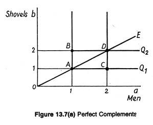
While discussing the nature of long-run produc­tion, Samuel Webb has drawn a distinction between substitute and complementary inputs. According to him, “in production processes where exact amounts of two or more inputs are required to produce given units of output, the inputs are said to be perfect complements.”

A classic example is the primitive case where one man plus one shovel can produce a hole in the ground in a given amount of time.

This is shown by point A on isoquant Q₁ in Fig. 13.7(a). An additional shovel, at point B, is of no value to a man who can use only one at a time. In a like manner, an additional worker where there is only one shovel at point C can produce no more holes, assuming shovels are essential for digging and that a worker can work continuously without relief.

We see that isoquants for perfect complements are Z-shaped. Other examples given by Webb include component parts such as frames and wheels for ve­hicles, leather and buckles for leather belts, han­dles and blades for knives, foundations and roofs for houses, and so on.

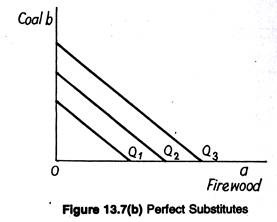
Some products can be produced by inputs that can be readily substituted for each other, e.g., coal and firewood. These two items might be perfect substitutes for each other in the generation of heat. Similarly, two nickels will work as well as one dime in operating many vending machines.

Alternative foods may fulfil minimum nutrient requirements equally well; for instance, peanut butter and corn meal are both rich in protein, white potatoes and – spinach are good sources of ascorbic acid. Ship­ments may be made as quickly by river as by rail. Isoquants for such examples are shown in Fig. 13.7(c).

In-between these two extreme cases there lie the more common cases where factors are substitutable for each other in varying degrees.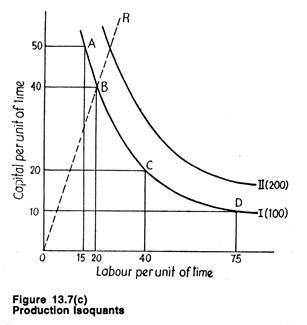

Fig. 13.7(c) illustrates two such isoquants. Iso­quants I indicates all possibly combinations of cap­ital and labour that are capable of producing the same level of output. We see that the firm can pro­duce 100 units of output by using 10 units of capital and 75 of labour (point D), or 50 units of capital and 15 of labour (point A), or by using any other combination of capital and labour specified by iso­quant I.

In a like manner, isoquant II shows vari­ous combinations of capital and labour that can be used to produce 200 units of output. However, each capital-labour combination can be on only one,iso­quant. In other words, isoquants, like consumption indifference curves, cannot meet or intersect. Iso­quants I and II are only two of an infinite number of isoquants that could possibly be shown in the di­agram.

All the isoquants together constitute an isoquant map In an isoquant map, an isoquant which lies above and to the right of another shows a higher level of output. Thus, in Fig. 13.7(c) isoquant II indicates a higher level of output than that indicated by isoquant I.

Distinguishing between Movements along and Movements among Isoquants:

Each of the two isoquants in Fig. 13.7(c) repre­sents the various combinations of the two variable inputs that can be used to produce the specified level of output. As we move from A to B along the iso­quant for 100 units of output, the only change is in the capital labour ratio.

At point B, we have more labour and fewer units of capital than at point A. Moving outward along a particular ray (like OR), the ratio of the two inputs remains constant, but to­tal output increases because more of both the inputs are being utilized.

Technical Vs. Economic Efficiency:

It is also important to note that combinations other than those on a given isoquant can be used to produce the given level of output; but such com­binations would not reflect the “maximum-amount- of-output” and thus show economic efficiency of the production process. In Fig. 13.7(c), it- is clear that 100 units of output could be produced using more than 10 units of capital and more than 75 units of labour.

However, such production would simply ‘waste’ economic resources. By contrast, it is im­possible to produce 100 units of output using less than 10 units of capital with 75 units of labour, or vice versa. For any combination along an isoquant, if the usage level of either input is reduced and of the other is held constant, output will fall.

The Marginal Rate of Technical Substitution:

As shown in Fig. 13.7(c) isoquants slope down­ward over the relevant range of production. This negative slope indicates that if the firm reduces the amount of capital employed, more labour has to be used to keep the level of output unchanged.

Al­ternatively, if labour use is decreased, capital usage must be increased to keep output constant. Thus, the two inputs can be substituted for each other to maintain a specified or fixed level of output.

The rate at which one input must be substituted for another keeping output constant, as along an iso­quant, is called the marginal rate of technical substi­tution (MRTS), and is expressed as

MRTS = ∆K/∆L

The minus sign is added in order to make MRTS a positive number, since ∆K/∆L, the slope of the isoquant, is already negative (because addi­tional use of any factor always at the expense of the other).

Over the relevant range (i.e., economic region) of productions the MRTS diminishes. That is, as more and more labour is substituted for capital keep­ing output constant, the absolute value of ∆K/∆L falls. This can be seen in Fig. 13.7(c).

If capital is reduced from 50 to 40 (a decrease of 10 units) labour must be increased by only 5 units (from 15 to 20) in order to keep the level of output unchanged at 100 units. That is, when capital is abundant rel­ative to labour, the firm can discharge 10 units of capital but must substitute only 5 units of labour in order to obtain the same level of output.

The marginal rate of technical substitution in this case is -∆K/∆L = (—10)/5 = 2, implying that for ev­ery unit of labour added, two units of capital can be released in order to maintain the same level of out­put. However, consider a combination where capital is more scarce and labour more abundant.

For ex­ample, if capital is reduced from 20 to 10 (again a reduction of 10 units) labour has to be increased by 35 units (from 40 to 75) to keep output unchanged at 100 units. In this case MRTS is 10/35, indicat­ing that for each unit of labour added capital can be decreased by 2/7 of a unit.

Thus, as capital is reduced and labour is in­creased along an isoquant, the amount of capital that can be released for each unit of labour added gradually diminishes. Differently put, the amount of labour that must be added for each unit of capital discharged, keeping output constant, must increase.

The slope of the isoquant measures the rate at which labour can be substituted for capital and vice-versa. It is observed that the isoquant becomes flatter and flatter as the producer moves downward from left to right. In other words, M RTS declines along an isoquant.

Relation of MRTS to Marginal Products:

By using elementary calculus we can summa­rize this relation very quickly. In the case of two- input production function

Q = Q (K, L)

we take the total differential and hold output con­stant on a particular isoquant. By using elemen­tary calculus we can summarize this relation very quickly. In the case of two-input production func­tion

In the theory of consumer demand we noted that MRS is the ratio of the two marginal utilities. The same type of relation holds here, too. Thus, for very small movements along an isoquant, the MRTS is just the ratio of the marginal products of the two inputs. This point may now be proved.

The level of output, Q, depends upon the use of the two inputs, L and K. Since output Q is the same at all points on an isoquant, ∆Q is zero for any change in L and K along an isoquant. Suppose that, at a point on the isoquant, the marginal prod­uct of capital (MPk) is 3 and the marginal product of labour (MP_L) is 6.

Then, if we add one unit of labour, output would increase by 6 units. How much capital must be eliminated to keep output un­changed? Capital must decrease enough to offset the increase in output generated by the increase in labour. Since the marginal product of capital is 3, two units of capital must be released. Thus, in our example, the MRTS = -∆K/∆L = – (-2)/1 = 2, which is exactly equal to MP_L/MP_k = 6/3 = 2.

Alternatively, if we were to reduce capital by one unit, output would fall by 3 units. Labour has to increase by ½ of a unit of neutralize the decline of 3 units of output or to keep output constant, since MP_L = 6. In this case the MRTS = -∆K/∆L = — (—1)/1/2 = 2, which is once more equal to MP_L/MP_k.

Thus, in general, when L and K are allowed to vary marginally, the change in Q resulting from the change in the two inputs is the marginal product of L times the amount of change in L plus the marginal product of K times its change.

Thus in terms of symbols:

∆Q = (MP_L) (∆L) + (MP_k) (∆K).

In order that the producer stays on the same isoquant it is necessary to set AQ equal to zero. Then solving for the MRTS, we get:

MRTS = ∆K/∆L = MP_L/MP_K

The M RTS diminishes as the producer moves along an isoquant from left to right. It is because as additional units of labour are substituted for capi­tal, the marginal product of labour falls.

Two forces work further to cause marginal product of labour to a fall:

(1) Less capital causes a downward shift of the marginal product of labour curve, and

(2) Ad­ditional units of the variable input (labour) cause a downward movement along the marginal product curve.

Thus, as labour is substituted for capital the marginal product of labour has to fall. For similar reasons, the marginal product of capital increases as less capital and more labour are used to produce the same level of output.

Thus, as labour is substi­tuted for capital the marginal product of capital in­creases. Combining these two conditions as labour is substituted for capital, MP_L decreases and MP_k increases; so MP_L /MP_k will diminish.

Ridge Lines and the Economic Region of Production:

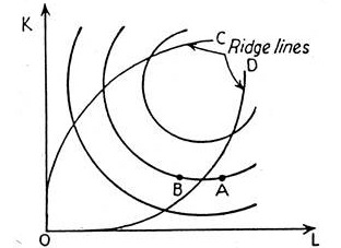
We have postulated convexity of isoquants. And it presupposes positive marginal product of L and K. But MP of L may become negative if the application of L is so large relative to quantities of other input(s), say capital, that an increase of labour would result in congestion and inefficiency, in which case MP may turn out to be negative. Then returns to scale (RTS) would become negative, as at point A of Fig. 13.7.

The definition of production function does not preclude the possibility of negative RTS. Clearly, a movement from A to B would result in a reduction of both L and K. And since inputs are to be paid, an entrepreneur would prefer point B to point A, as he is assumed to behave rationally. The ridge lines OC and OD enclose the area of rational operation, i.e., they delineate the regions in which input combinations are economical.

Figure 13.8

Ridge Lines

The Optimal Combination of Inputs:

Thus it is clear that any desired level of output can be produced by a number of different combina­tions of inputs. But as we noted at the outset, one of the four production decisions a manager must make is: which input combination to use, or, what is the ‘optimal’ input combination?

The manager can choose from among different combinations of capital (K) and labour (L) to pro­duce a given level of output. Or, faced with spec­ified input prices, it can choose from among many combinations of K and L that would lead to a fixed level of cost, i.e., expenditure.

Thus he has to make either of two input choice decisions:

1. Choose the input combination that yields the maximum level of output possible with a fixed out­lay (i.e., output maximization subject to cost con­straint).

2. Choose the input combination that leads to the lowest cost of producing a fixed level of output (i.e., cost minimization subject to output constraint).

The solution to any constrained maximization or minimization problem is choosing the level of each activity whereby the marginal benefits from each activity, per rupee spent, is the same at the margin.

To ensure this, the profit-maximizing firm has to choose that input combination for which the marginal product divided by input price is the same for all inputs used. The implication is that for our two-input case a firm attains the highest level of out­put when

MP_L/P_L = MP_k/P_K or MP_L/w = MP_K/r

were w and r are, respectively the prices of labour (P_L) and capital (P_K). Thus the MRTS = (MP_L/ MPk) equals the factor price ratio (w/r). This com­bination may now be illustrated graphically.

Input Prices and Isocosts:

The isoquant shows the desire of the producer. But the desire to produce a commodity is not enough. The firm must have capacity to do so. Usually a firm is supposed to have a fixed amount of money to buy resources. In other words, like a consumer, the pro­ducer has also to operate under a budget constraint. The isocost line is, in fact, the producer’s budget line.

In determining the optimal input combination, a profit-maximizing firm or producer has to pay at­tention to relative input prices if it is to minimize the cost of producing a given output, or maximiz­ing output for a given level of cost. Input prices are determined by the market forces, i.e., by sup­ply and demand in the input market.

For producers who are not ‘monopsonists’ or ‘oligopsonists’ (i.e., the sole purchaser of, or one of a few purchasers of an input), input prices are taken as given by the mar­ket. Here we look at a producer who is a competitor in the input market facing given market-determined input prices; so we treat the input prices as fixed.

So the total cost equation is C = rK + wL where all the terms have their usual meaning. Total cost (outlay) is simply the sum of the cost of K units of capital at r rupees per unit and of L units of labour at w rupees per unit.

Let us consider a simple example. Suppose cap­ital costs Rs. 100 per month per unit (r = Rs. 100) and labour receives a wage of Rs. 250 per unit (w = Rs. 250). Then the firm’s total cost function is

C = 100 K + 250 L.

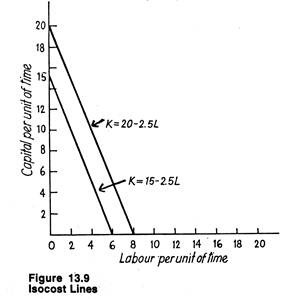
Now suppose the firm decides to spend Rs.1, 500 per month for capital and labour. Thus the equation becomes 1500 = 100A’ + 250L . If we solve this equation for K, we see the combinations of K and L that can be chosen is K = 15 — 2.5L.

Similarly, if Rs. 2,000 are to be spent on K and L, the firm can purchase combinations given the relation: K = 20 — 2.5L. In a more general situation, if a fixed amount C is to be spent, the firm can choose among the combinations given by

This equation is illustrated in Fig. 13.9. If Rs. 1,500 is spent on capital alone, 15 units of capital may be bought. If Rs. 2,000 is spent on capital alone, 20 units of capital may be purchased.

More generally, if C is to be totally spent and r is the unit cost, the maximum amount of capital that can be purchased is C/r units; C/r is, therefore, the vertical intercept of the line. If one unit of labour is purchased at Rs. 250, 2 ½ units of capital have to be sacrificed; if 2 units of labour are bought, 5 units of capital must be given up and so on.

Thus, as the purchase of labour is increased, the purchase of capital has to fall if total cost remains fixed. In other words, each extra unit of labour purchased, w/r units of capital must be foregone. In Fig. 13.9, w/r = 2.5. The negative of this ratio is the slope of the line. This slope shows the actual rate of fac­tor substitution, i.e., the rate at which capital can be substituted by labour, or labour by capital, in the market-place.

The lines in Fig. 13.9 are called isocost lines be­cause they show the various combinations of in­puts that may be purchased with a fixed amount of money. In other words, total cost is the same at all points on the line.

An increase in outlay, holding factor prices fixed, leads to a parallel rightward shift of the isocost line. Thus the isocost line for C = Rs. 2,000 lies above the line for C = Rs. 1,500. There would exist an infinite number of isocost lines, each relating to a different level of cost outlay (expenditure).

At fixed input prices, r and w for capital and labour, it is possible to purchase with a fixed outlay C, any combination of capital and labour given by the following linear equation:

K = C/r – w/r L.

This is the equation for an isocost line whose intercept (C/r) is the amount of capital that may be purchased if no labour is bought and whose slope is the negative of the factor-price ratio (w/r).

If the relative factor prices change, the slope of the isocost line must change, If w rises relative to r, the isocost line becomes steeper. If w falls relative to r, the isocost line becomes flatter.

Production of a Given Output at Minimum Cost:

Whatever output a firm chooses to produce, the production manager is desirous of producing it at the lowest possible cost. To accomplish this objec­tive, the production process must not only be tech­nically efficient but economically efficient, as well. So the production process has to be organized in the most efficient manner.

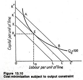
Suppose that at given input prices r and w, a firm wishes to produce the output indicated by isoquant Q₀ = 100 in Fig. 13.10. Isocost lines KL, K’L’ and K”L” are three of the infinite num­ber of isocost lines from which the producer can choose at the given factor prices. Obviously, the firm will choose the lowest level of cost outlay that en­ables output level Q₀ = 100 to be produced.

In Fig. 13.10 that output level will be produced at the cost represented by isocost line K’ L’. Any cost out­lay below that, for example that represented by KL, is not feasible since it is impossible to produce out­put Q₀ with these factor combinations. Any factor combination above that represented by K’L’ are not considered because the firm seeks to produce the de­sired output at least cost.

If combinations A or B are chosen, at the cost outlay represented by K”L”, the producer can reduce costs by moving along Q₀ to point E. Point E shows the optimal resource combination, K₀units of capital and L₀ units of labour. This is known as the least cost combination (i.e., most efficient) of inputs.

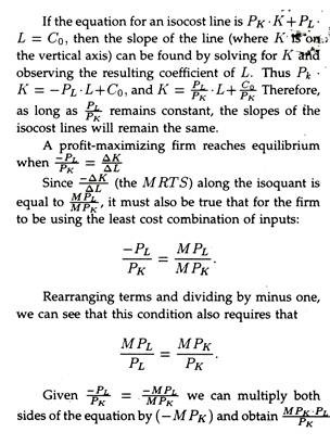
Recall that the isoquant shows the desired rate of factor substitution and the isocost line the actual rate of factor substitution. A firm reaches equilib­rium and thus minimizes cost when the lowest pos­sible isocost line (whose slope is the factor-price ra­tio) is tangent to the isoquant (whose slope is MRTS).

At this point of tangency the slopes of the two curves are equal, or,

MP_L/MP_k = w/r, or, MP_L/w = MP_k/r

Put differently, production at least cost requires that the MRTS of capital for labour be equal to the ratio of the price of labour to the price of capital.

The factor price ratio tells the producer the rate at which one input can actually be substituted for another in the market place. Recall that MRTS shows the rate at which the producer can substitute between the inputs in production. If the two are not equal, a firm can reduce cost further by altering the factor proportion.

Thus, to minimize the cost (expenditure) neces­sary to produce a given level of output with given input prices, the producer must combine inputs in such quantities that the MRTS of capital for labour is equal to the factor price ratio (the price of labour to the price of capital).

We can analyse the equilibrium condition in an alternative way. Suppose the equilibrium condition did not hold or, specifically, that the producer was at point B in Fig. 13.9. At point B,

In this case the marginal product of an addi­tional rupee worth of labour is less than the marginal product of an additional rupee worth of capital. The firm could therefore reduce its use of labour by Re. 1, expand its use of capital by Re. 1, and produce the same level of output but at a reduced cost. It could continue to do this until the above inequal­ity is converted into an equality.

Eventually, MP_L /w would become equal to, MP_k/r since MP_L rises with decreased use of labour and increased use of capi­tal and MP_k falls with increased capital, and de­creased labour. By following the same logic it is pos­sible to establish that if the inequality is reversed, such as the case at point A, the firm would con­tinue to substitute labour for capital until the equal­ity holds.

Mathematical Note:

This equation states that for the firm to be em­ploying the least cost combination of inputs K and L, the additional output obtainable from spending an extra rupee on input L must equal the additional output obtainable from spending another rupee on input K.

If this relationship did not hold, the firm would gain by purchasing less of the input with a lower additional output per additional rupee expen­diture, and more of the input with a greater additional output per extra rupee expenditure.

Example:

Suppose for a firm using two inputs K and L, MP_L = 5, P_L = Rs. 5, MP_K = 40, and P_K = Rs. 25. Is the firm optimizing the use of its resources? If not, why not?

Solution:

Here MP_L /P_L < MP_K /P_K (1unit per rupee < 1.6 units per rupee). So the firm would be better off by using less labour and more capital. (If the firm spend an additional Rs. 25 on labour it would gain 25 units of output, whereas if it spends an additional Rs. 25′ on capital, it would gain 40 additional units of output).

Production of Maximum Output with a Given Level of Cost:

An alternative, but more preferable way of pre­senting the optimization problem is to assume that the firm can spend only a fixed amount of money to produce a commodity and it seeks to attain the high­est level of production consistent with that amount of outlay. This approach seems to be more practical than the previous one. The end result will be the same as before.

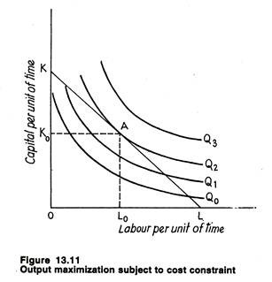
Such a situation is illustrated in Fig. 13.11. The isocost line K_L shows all possible combinations of the two inputs that can be purchased with a fixed amount of money and a fixed set of factor prices. Four hypothetical isoquants are shown. Clearly, at
the given level of cost, output level Q₃ is unattain­able. And, neither output level Q₀ nor level Q₁ would be chosen, since higher levels of output can be produced with the fixed cost outlay. The high­est possible output with the given level of cost is produced by using L_o amount of labour and K₀ amount of capital.

At point A, the given isocost line is tangent to the highest attainable isoquant, viz., isoquant Q₂. Thus, in the case of constrained out­put maximization, the MRTS of capital for labour equals the factor-price ratio (the price of labour to the price of capital).

Thus in order either to maximize output sub­ject to a given cost or to minimize cost subject to a given output, the production manager must employ factors in such amounts as to equate the MRTS with the factor price ratio.

The Expansion Path:

In Fig. 13.11 we illustrated one optimizing point for a firm. This point shows the optimal (least cost) combination of inputs for a fixed level of output.

However, we know that there exists an optimal com­bination for every level of output the firm might choose to produce, and the proportions in which the inputs are combined need not necessarily be the same for all levels of output. To examine several optimizing points at a time we use the expansion path.

The expansion path shows the way in which fac­tor proportions change in response to output changes, with the factor-price ratio remaining unchanged. In Fig. 13.12 the curves Q₀– Q₁ and Q₂ are isoquants depicting a representative production function.

The isocost lines KL, K’L’ and K”L” represent the minimum costs of producing each of the three out­put levels, since they are tangent to the respective isoquants. Since we do not assume any change in the factor-price ratio up to this stage, these isocost lines are parallel.

Look at the three optimum points, A, B, and C. Since at each of these:

(1) Factor prices remain con­stant, and

(2) The MRTS is equal to the factor-price ratio, it follows that the marginal rates of technical substitution are equal at A, B, and C.

Therefore, the expansion path, OS, is a locus of points along which the MRTS is constant and equal to the factor price ratio. But it is a curve having a special feature: It is the locus along which output will expand when fac­tor prices are constant. We may accordingly suggest a definition.

The expansion path is the curve along which the firm expands (or contracts) output when fac­tor prices remain constant. It indicates how fac­tor proportions change when output (or expendi­ture) changes, factor prices remaining unchanged.

It shows output expansion effect which is similar to income effect (studied in the theory of consumer demand). Since it is made up of points of efficient (least cost) input combinations, the expansion path is the locus of efficient combinations of the in­puts. On the expansion path, the MRTS remains constant, since the factor-price ratio is constant.

The expansion path gives the firm its cost structure. In fact, the long-run total cost curve is derived from the expan­sion path. The expansion path shows the optimal (least-cost) combination of inputs to be used to pro­duce each level of output.

The sum of the quantities of each input used, times the respective input price, gives the minimum cost of producing every level of output. This is turn allows us to relate cost to the level of output produced.

Changes in Relative Prices:

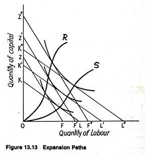
We have derived the expansion path under only one set of input prices. But, it should be clear that change in relative input prices change the expan­sion path and hence the cost structure. For exam­ple, consider first the expansion path OS shown in Fig. 13.13.

The relative price of capital and labour is given by the slope of KL, K’L’, K”L”. The tangencies of these isocost lines to isoquants Q₀, Q₁ and Q₂ indicate the optimal quantities of capital and labour used to produce each of these three levels of output and OS, of course, gives the optimal combi­nation for every level of output over the range.

Now, suppose the price of labour (or wage rate) increases relative to the price of capital (or the rate of interest). Since the ratio w/r increase, the iso­cost lines become steeper. These new isocost lines are shown as ZF, Z’F’ and Z” F”. Now the tangency on each isoquent occurs at a smaller quantity of labour and a large quantity of capital.

These new optimal combinations indicate that the firm substi­tutes capital for labour to produce each level of out­put when the price of labour rises relative to the price of capital. This is called the input (factor) sub­stitution effect. It results from a change in factor prices. So the new expansion path, OR, is estab­lished and it shows the new optimal combination of inputs for each level of output.

Further changes in factor prices would lead to further factor substitution. The direction of substi­tution depends upon the nature and direction of the relative change in factor prices. If the price of labour rises relative to the price of capital, the firm substi­tutes capital for labour at each level of output, and production process becomes more capital intensive (e.g., tractorisation in agriculture or computerisation in industry).

If the price of capital rises relative to the price of labour, the firm substitutes labour for capital (e.g., manual operation of petro pumps in place of power-driven machines). Firms will always substitute away from the input that becomes rela­tively expensive towards the input that becomes rel­atively cheap.

So long we have focused on production un­der variable proportions. But, a production func­tion could also be characterized by production under fixed proportions. For example, if 2 units of labour and 5 units of capital are necessary to produce 100 units of output, 200 units of output require 4 of the labour and 10 of capital, 300 units require 6 of labour and 15 of capital, and so on. If labour is limited to 2 units, no matter how much capital is added beyond 5 units, only 100 units of output can be produced. In this case the capital to labour ratio, K/L is always 5/2, regardless of the level of output.

All fixed proportions production functions are characterized by a constant factor proportion (or K/L ratio) at every output level. In this fixed fac­tor proportion case, the isoquants will be L-shaped and the expansion path is a straight line through the origin.

This means that if labour remains at a given level while capital is increased, no more output can be produced. Neither can an increase in labour raise output if the stock of capital remains unchanged. It, therefore, follows that no matter what the ratio of input prices is, the firm uses the same combination of inputs to produce each given level of output. In this case the input substitution effect is absent.

Elasticity of Factor Substitution:

A complex concept, the elasticity of substitu­tion, is a property of production function. It is a measure of the ease or difficulty of substituting cap­ital for labour in response to a change in the ratio of the prices of labour and capital. In some pro­duction functions the elasticity of substitution is as­sumed to be unity; many empirical studies (such as those made by Cobb and Douglas) have also shown values close to unity.

This implies that a 1% increase in the ratio of the price of labour to the price of cap­ital causes a 1% increase in the capital-labour ratio. The elasticity of substitution is also important in an analysis of the relative shares of labour and capital in the national product (income).

Mathematical Note:

The slope of the isoquant indicates the substi­tutions that, if made, will leave output unchanged. Hence the slope of the isoquant through any point becomes

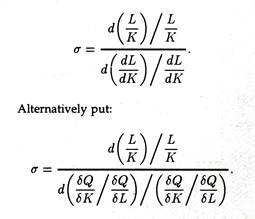
The numerical value of this slope is termed the marginal rate of substitution of the services of factor L for those of factor K and reflects the relative ease of substituting the services of factor L for those of factor K. The relative change in the marginal rate of substitution is called the elasticity of substitution. The elasticity of substitution may be expressed as

Finally, assuming that the ratio of factor prices is equal to the ratio of marginal products, we get

Thus, the elasticity of substitution, as defined by Sir John Hicks, is a measure of the relative change in the factor proportion divided by the relative change in factor-price ratio.

Returns to Scale:

In the short run we study the returns to a fac­tor. In the long-run we study returns to scale. In the long-run all factors are variable and it is possible to change the scale of production of the business firm.

We may now consider the effect of a proportionate increase in all inputs, on the level of output pro­duced. For example, if we were to double both K and L inputs, output would surely increase but we do not know by how much. To answer this question, we need the concept of returns to scale.

Let us consider an increase in the usage of all inputs by a proportion a. If output increases exactly by the same proportion, the production function is said to exhibit constant returns to scale.

If, however, output increases by more than a, production func­tion is said to exhibit increasing returns to scale. Al­ternatively, if output increases by less than a, the production function is said to be characterized by decreasing returns to scale.

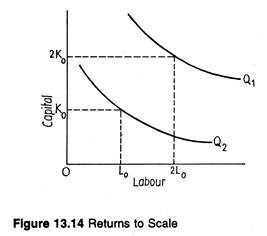
These relations can be illustrated, using Fig. 13.14. We start with an arbitrary level of usage of capital and labour at K₀ and L₀. This combi­nation of capital and labour produces some level of output, Q₀ = 100 units. Now, we double our level of inputs to 2K₀ and 2L₀ and, as a result, output increases to Q₁.

If Q₁ is exactly equal to 200, this is a case of constant returns to scale. If Q₁ is greater than 200 units (say, 215), there is increasing return to scale. Finally, if Q₁ is less than 200 units (say, 180) the production function is said to exhibit decreasing returns to scale.

The returns to scale may be treated more an­alytically by expressing the production relation in functional form as

Q = ƒ(L,K).

Suppose we increase the inputs by a constant proportion (say, a) and output gets multiplied by αⁿ. Then we have

αⁿQ = ƒ(α L, αK).

Here α and αⁿ represent increases in the scale of operation and level of output, respectively. We have noted, in the case of constant returns to scale, if inputs are increased by a given proportion, output rises by the same proportion, that is, αⁿ= a.

More generally, if all inputs are increased by a factor a and output gets multiplied by a factor of αⁿ then a firm experiences:

1. Increasing returns to scale if n > 1, in which case αⁿ > α (output goes up proportionately more than the increase in input usage).

2. Constant returns to scale if n = 1, or αⁿ = α (output goes up by the same proportion as the increase in input usage).

3. Decreasing returns to scale if n < 1, or αⁿ < α (output goes up proportionately less than the increase in input usage).

Returns to Scale and Cost Behaviour:

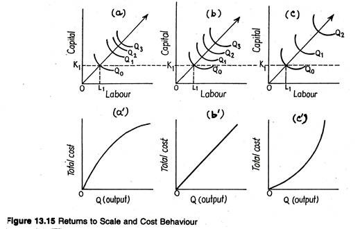
An intuitive understanding of the concepts of increasing, constant and decreasing returns to scale can be developed by looking at Fig. 13.15. Suppose we start with a given capital/labour ratio of K₁/L₁, which is the same in all the three panels.

The ques­tion to be answered about returns to scale is: How much do we have to increase the two inputs, capital and labour, in order to keep on doubling the rate of output from Q₀ to Q₁, Q₂ to Q₂, and Q₂ to Q₃.

In panel (a) of Fig. 13.15, increasing returns to scale is illustrated. This can be verified by compar­ing the respective distances between the isoquants along the ray emanating from the origin. We know that along any ray from the origin, the ratio of the two inputs remains constant.

Since here we are in­terested in analysing the case of proportional changes in all inputs, we have only to compare the dis­tances between the isoquants as measured along the ray from the origin. The rays through the origin in all the three panels have equal slope.

In panel (a) the distance along the ray from the origin to the first isoquant (Q₀) exceeds the distance between the first isoquant (Q₀) and the second isoquant (Q₁), which exceeds the distance between the second (Q₁) and the third (Q₂), and so on. Thus, it is possible to double output by less than doubling of inputs.

Panel (b) illustrate the case of constant returns to scale. In this case the distance along the ray between any two successive isoquants remains unchanged, suggesting a proportionate increase in both inputs and output. Differently put, a doubling of the in­puts will lead to a doubling of output.

Panel (c) shows decreasing returns to scale. The distance be­tween successive isoquants gets larger and larger for proportionate increases in inputs. That is, the pro­duction process demands more than a doubling of all inputs in order to exactly double the level of out­put.

Because all inputs have a cost, the long-run con­cept of returns to scale has significant implications for the behaviour of the long-run cost curve, and these results are shown in panels (a’), (b’), (c’) in Fig. 13.15. We shall deal more completely with the linkage between returns to scale and long-run costs. Here, Fig. 13.15 highlights the nature of the inverse relationship between produc­tivity and cost.

Thus, constant returns in panel (b) leads to linear total cost curve in panel (b’) – constant cost per unit. In like manner, increasing returns in panel (a) results in total costs in panel (a’) growing at a decreasing rate, that is, continuously declining cost per unit. Finally, decreasing returns in panel (c) leads to a total cost curve in panel (c’) with a constantly increasing slope, or constantly increasing cost per unit.

Reasons for Increasing and Decreasing Returns to Scale:

There are various variables that might account for the phenomenon of increasing returns to scale. As a firm expands the scale of its operation, oppor­tunities for increased specialization in the use of re­source inputs normally occur. This point was first made by Adam Smith in his The Wealth of Nations where he analysed the production process in a pin factory.

Rather than each worker making a complete pin, increased output allows workers to divide up tasks into separate activities, such as drawing the wire and forming the pin.

Transportation costs are also likely to be affected by the size of the firm. Typically, transportation costs are related to the size of the market. Trans­portation costs do not double when the size of the market gets doubled. Firms can also take advan­tage of large-scale equipment due to indivisibility of factors.

As noted by Bails and Peppers, “a construc­tion firm may be able to utilize more fully larger and more efficient equipment, than would a smaller construction firm. The most probable explanation for decreasing returns to scale is that there are lim­its to the effective management of larger and larger production units. As the layers of management in­crease, lines of communication become blocked and the ability to make prompt management decisions hindered”.

Economies of Scope:

Economies of scope exist for multiple products when the cost of joint production is less than the cost of producing each output separately. In other words, as Pappas and Brigham have put it, “a firm will pro­duce products that are complementary in the sense that producing them jointly is less costly than indi­vidual production”.

This concept explains best why firms produce multiple rather than single products. This new concept forces management to con­sider both direct and indirect benefits associated with individual lines of business. For example, on a product line basis, some firms offer products as a “loss leader”.

Economies of scope assume added significance of late because they permit a firm to translate supe­rior skill or productive capability in a given prod­uct line into unique advantages in the production of complementary products.

In terms of business pol­icy, this suggests that an effective competitive strat­egy would be one emphasizing the development or extension of product lines related to a firm’s well established products.

For example, USA’s Pepsi Co. Inc., has long been a leader in the soft drink world. Over an extended period of time, the Company has gradually broadened its product line to include var­ious brands of snack food like corn chips.

This product line extension strategy was effective because it capitalized on the product development capabili­ties, distribution network, and marketing skills de­veloped by the firm in its soft drink business. This has led to considerable cost saving.

In this context, Pappas and Brigham have com­mented that “the economies of scope concept plays an important role in managerial decision making be­cause it offers a useful means for evaluating the po­tential of current and prospective lines of business. It naturally leads to a definition of those areas in which the firm has a comparative advantage and thus its greatest profit potential”.

Testing Production Functions for Returns to Scale:

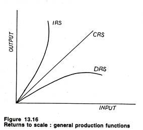
Fig. 13.16 illustrates the generalized relation­ship between the level of output and the level of input usage (with the factor mix of labour to capi­tal held constant). It is possible to identify returns to scale.

Suppose that we start with the following production function:

Q = f(X₁, X₂, X₃). (1)

Furthermore, suppose that we multiply each in­put by a constant a. Due to the proportionate in­crease in all inputs, output will increase by some proportion, which, by convention, we will call A.

In terms of the above production function we get:

λQ = ƒ(αX₁, aX₂, aX₃).

To test production functions for returns to scale, all that is necessary is to compare the value of There are various variables that might account to the value of λ:

1. If λ> α, the production function exhibits increasing returns to scale.

2. If λ< α, the production function exhibits decreasing returns to scale.

3. If λ= α, the production function is characterized by constant return to scale.

For example, suppose that the following pro­duction function has been estimated as:

Q = 7X₁+4X₂+ 0.3X₃. (3)

Furthermore, suppose that the initial values of the inputs are X₁ = 2, X₂ = 1, and X₃ = 3. Based on these initial input values, total production would be

Q = (7)(2) + (4)(1) + (0.3)(3) = 18.9. (4)

Now suppose that we double the inputs to 4, 2 and 6, respectively. On the basis of these new input values, output becomes

Q = (7) (4) + (4)(2) + (.3)(6) = 37.8. (5)

In this case a doubling of inputs (α = 2) leads to an exact doubling of output (λ = 2). Thus, the original production function is characterized by con­stant returns to scale (λ =α).

Alternatively, consider the production function given below

Q = 2 K² + 6KL. (6)

If the initial values of K and L are 1 and 2, respectively, then total output is 14. If both inputs were doubled (α = 2), output would increase to 56(λ = 4). Output has quadrupled, indicating a production function exhibiting increasing returns to scale (λ > α).

The Degree of Homogeneity of a Production Function:

If the constant term a can be factored out of the production function, the function is said to be homo­geneous of degree n. For example, if the production function given in Eq. (7) is multiplied by the factor α, we obtain

Since α can be factored out of Eq. (7), and a in Eq. (8) has an exponent of 1, the production function in Eq. (8) is said to be homogeneous of degree one.

The general procedure of determining the ho­mogeneity of a production function is to utilize the following scheme and thus evaluate αⁿ:

1. If n > 1, we have increasing returns to scale.

2. If n < 1, we have decreasing returns to scale.

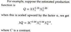
3. If n = 1, we have constant returns to scale. For example, suppose the estimated production function is

Because the exponent of α 0.58, is less than 1, the production function is characterized by de­creasing returns to scale.

Elasticity of Production:

An alternative procedure for testing for the pre­sence of returns to scale is to examine the elasticity of production, a concept introduced earlier. Because returns to scale is a relative measure – a comparison of the percentage increase in output usage relative to the percentage increase in all inputs – it corresponds

to an elasticity of production measure. If the elastic­ity of production coefficient exceeds 1, the produc­tion function shows increasing returns to scale; if it equals 1, there are constant returns to scale; and if it is less than 1, there are decreasing returns to scale.