The Shape of a Firm’s Cost Curves in Long Run and Short Run

Let us make an in-depth study of the shape of a firm’s cost curves in long run and short run.

Short Run Cost Curves:

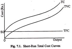
The cost schedules in Table 7.1 are represented graphically. Fig. 7.1. shows total fixed costs as a horizontal straight line at a figure of Rs. 50, because this cost is increased at all levels of output (starting with zero and ending with 10).

The curves TC and TVC are parallel. The vertical distance between them is Rs. 50, which is TFC.

Thus, we find that as output increases the average cost decreases. This will hold good up to the point of maximum capacity of the equipment and scale used in the factory. If production is pushed beyond this level, without changing the equipment and scale, difficulties will arise.

More intensive utilisation of the fixed equipment must necessarily lead to diminishing returns. Overtime allowance will have to be paid; the work period will have to be lengthened out into double or triple shifts. In effect there will be increase in the use of labour and raw materials while capital equipment is kept constant. The law of variable
proportions will apply and diminishing returns or increasing costs will begin to operate.

Thus, in the short run we find that as output increases the average cost falls up to the point of maximum capacity of the equipment and scale used in the firm and rises thereafter. The average cost curve is U-shaped, falling to a minimum and there­after rising.

The marginal cost curve will follow the average cost curve because they are related in a definite way. The marginal cost falls for initial increases of output and thereafter increases continuously.

Diagrammatic Illustration:

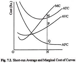
The short-run cost curves can be diagrammatically represented as in the figure below:

The curve AFC shows the average fixed cost. It must slope downwards to the right because as output increases the average fixed cost diminishes. The curve AFC is a rectangular hyperbola because average fixed cost x quantity produced = a constant.

The curve AVC shows the average variable cost. It slopes downwards in the initial stages but thereafter rises slowly. The curve ATC shows average total cost. The ordinates of ATC are obtained by adding up the ordinates of AVC and AFC, i.e., if P, Q and M are corresponding points on the three curves, PN + QN = MN. The curve MC shows marginal cost.

Fig. 7.2 shows the four short-run cost curves of an individual firm. ATC is the curve of average total costs. It slopes downwards initially and then rises upwards.

The following points are to be noted:

(i) The short-run average cost curve may be like a U or a V or like a ‘dish’, depending on the nature of the equipment and scale and their productivity. The relative lengths and inclinations of the upward and the downward portions of the curve differ from firm to firm and industry to industry. Generally speaking, the shape of the curve depends on the relative importance of the fixed and the variable costs of production and the degree of sharpness with which the law of diminishing returns is operative for the variable factors.

(ii) The curves show cost changes brought about by changes in output, other things remaining the same.

(iii) Cost changes may be due to extraneous factors, e.g., rise in the price of raw materials, increase of wages, etc. Such changes will be shown by shifting the curves to new positions.

The Relation (a) between AP and AVC and (b) between MP and MC:

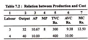
There is a close relation between production and costs. To explain the relation between the two in the short run let us assume that there is only one variable factor, labour. Columns 2,3 and 4 of Table 7.2 gives us figures of total product, average product and marginal product for three and four units of labour. Here total product is, respectively, 32 and 40 units. The AP and MP figures are given in columns 3 and 4.

Suppose the wage rate is Rs. 100 per worker. Then if 3 workers are employed total output is 32 units and TVC is Rs. 300, shown in column 5. Similarly, when 4 workers are employed TVC = Rs. 500 and total output is 40 units. So the AVC at an output of 40 units is TVC/Q = Rs. 400/40 = Rs. 10.

Table 7.2: Relation between Production and Cost

It is possible to write total variable cost as the price per worker, Rs. 100, multiplied by the number of workers, four. We can also write total output, Q, as the average product, 10, multiplied by the number of workers, four.

Thus, we can define average variable cost as:

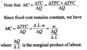
A similar relation can be shown between marginal cost and marginal product. The marginal cost of adding an additional worker to produce an additional 8 units of output is ATVC/AQ = Rs. 100/8 = Rs. 12.50. It may be noted that the change in variable cost from producing the additional 8 units of output is the cost of hiring the additional unit of labour, Rs. 100. The additional output is simply the marginal product of the additional worker, 8.

Thus we can write marginal cost as:

MC = w/Mp = Rs. 100/8 = Rs. 12.50.

Thus, we see that when only one input is variable in the short run, the following relations must hold:

AVC = w/AP and MC= w/MP.

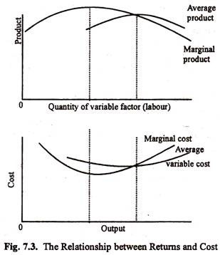
From these relations, it is possible to determine the shapes of the average variable cost and marginal cost curves. When average product of the variable factor (labour) is increasing, average variable cost is decreasing. When average product of labour is decreasing, AVC is increasing. Therefore, since average product first increases, reaches a maximum, then decreases, average variable cost first decreases, reaches its minimum (when average product attains its maximum), then increases.

The shape of the average product curve leads to a U-shaped AVC curve. Thus the AVC curve is U-shaped because of the Law of Variable Proportions which states that if all inputs cannot be increased proportionately output will follow the Law of Non-proportional Returns. Since the shape of ATC is deter­mined by the shape of AVC, the ATC is U- shaped because of the Law of Variable Proportions.

From the second relation, as marginal product rises, marginal cost falls; when marginal product declines, marginal cost rises. Marginal cost attains its minimum point when marginal product attains its maximum. Therefore, the shape of the marginal cost curve in the short run depends on the shape of the marginal product curve of the variable factor (labour in our example).

If it increases marginal cost will fall and vice versa.

Here we assume that only two factors are being used—one is fixed factor (say capital). If each unit of the variable factor costs the same, but the output from additional units is increasing, the firm is obtaining an increasing output for any given addition to expenditure.

In other words, the cost of each additional unit of output is falling as output expands. On the other hand, if the marginal product of the variable factor is diminishing, the cost of an additional unit of output is rising. This cost of an additional unit of output is known as marginal cost (MC).

The above points are illustrated diagrammatically in Figure 7.3, where average product = total product of n units of the variable factor/w, and average variable cost = total variable costs of n units of output/n.

The Relationship between Average Cost and Marginal Cost:

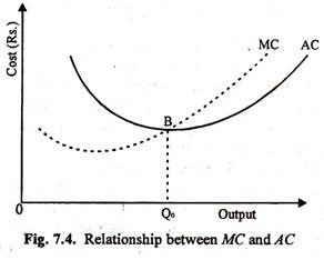
In Figure 7.2 we see that the MC curve cuts both the A VC curve and the ATC curve at then- respective minimum points. The relationship between ATC or, simply AC and MC is very close and requires further discussion.

In Fig. 7.4 we see that the MC curve cuts the AC curve from below at its lowest point.

The relationship is mathematical. A simple real life example will make this clear.

Suppose that a basketball team scores 80 points in its first game and 90 in its second. Its average score per game is therefore (80+90)/2, or 85 points per game—the total number of points scored in both games divided by the number of games. Now if the team scores less than the average in the third game, say 70, the average number of points scored per game will decline from 85 to (80+90+70)/3, or 80. On the other hand, if the team scored 100 points in the third game, the average number of points scored per game would increase from 85 to (80+90+100)/3, or 90.

The same principles applies in relation to the cost curves in Fig. 7.4. If MC is below AC, it pulls down the AC; if MC is above AC, it pulls up the AC. But when MC is equal to AC, the AC remains unchanged, i.e., it neither falls nor rises. Moreover, this must occur at the lowest point of the AC curve because it is at that point that the AC curve is neither is falling nor rising.

Long Run Average Cost Curves:

After discussion the short-run cost behaviour we may pass on to long-run cost behaviour. The short-run is the time period during which production cannot be fully adjusted to meet a change in demand because some of the factors cannot be varied. On the other hand the long-run is the period during which all types of adjustments can be made to meet the changed demand because all the factors can be varied.

Thus, if the demand for bus transport in a particular town increases greatly in the short run there should be greater use of the existing buses. But in the long run additional buses can be ordered. The long-run is the period when full adjustment can be made.

The same thing is true of a firm. In the short run extra output can be produced by a firm by utilising its existing capacity (i.e., plant and machinery) more intensively. In the long run, capacity can be varied, new machines can be ordered, the size of the factory can be altered, or new factories can be set up.

In the short run full adjustment to a change in demand is hindered by the fact that some of the factors are fixed in supply for the time being. On the other hand, a long run curve shows the cost per unit for different levels of output when all factors can be varied.

The U-shaped curve:

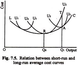
For a particular level of equipment and scale the average cost of a firm is represented by a U-shaped curve. Suppose U₁, U₂, and U₃ in Fig. 7.5, are three different short run average cost curves for three different scales of production. For each of these scales there is an optimum output. The producer would ordinarily like to produce the optimum output because his average cost is least at this point. But if demand changes it may be necessary to increase or decrease his output and he may consider it desirable to alter his scale of production.

Suppose at a particular time, a producer is under cost curve U₂ and produces OQ₀. He finds it necessary to produce OQ₁. If he continues under the old scale his average cost will be Q₁T. Suppose he alters his scale so that his new cost curve is U₃. The average cost of producing OQ₁ is now Q₁A. Q₁A is less than Q₁T. So the new scale is preferable to the old and will be adopted. In the long run the average cost has changed from Q₀R to Q₁A.

Relationship:

Relationship between the long-run cost curve and the short-run cost curves:

The long-run cost curve is a curve which shows how costs change when the scale of production is changed. This curve is obtained by drawing a line which touches the series of possible short-run cost curves. In Fig. 7.5 LRAC is such a line. Mathematically speaking LRAC is the envelope of U₁, U₂, U₃, etc.

The long-run cost curve is the locus of equilibrium point on the short-run cost curves. At the equilibrium points, a movement along the short-run cost curve and a movement along the long-run cost curve must involve the same change of cost. That is, the short-run and the long-run marginal costs must be equal. This condition is satisfied only if the long-run average cost curve is tangential to the short- run average cost curves.

Shape:

Shape of the Long Run Average Cost Curve. The general opinion is that the long-run average cost curve is U-shaped, like the short-run average cost curve, but is flatter.

This means three things:

(i) The long run cost curve initially slopes downwards, i.e., average costs fall.

(ii) Later on, it slopes upwards, i. e., average costs increase.

(iii) The rate of increase or decrease of costs is less than what they are in the short-run.

Proof:

These propositions can be proved as follows:

Initially the average cost decreases because certain economies of scale are available (the economies of large scale production; economical use of the indivisible factors of production, etc.). With expansion of scale a stage comes when no further economies are available or the economies are more than counter­balanced by, diseconomies (like managerial difficulties, higher transport costs, etc.).

When this stage comes the average cost begins to rise. In either case the rate of decrease or increase of costs is slower than file rates in the short run because fixed costs play a more important part in the short run. In the long run the fixed equipment can be altered. The equipment can be adjusted to the output. In the short run such adjustment is not possible and, therefore, costs vary considerably with variation of output.

E. Chamberlin observes that long-run average cost curve slopes downwards initially, primarily for two reasons:

(i) increased specialisation made possible in general by the fact that the aggregate of resources is larger and

(ii) qualitatively different and technologically more efficient units of factors, particularly machinery, made possible by a wise selection from the greater range of technical possibilities opened up by the greater resources.

These two explanations overlap substantially. After the minimum point is reached, the AC curve slopes upwards because of the greater complexity of the producing units as it grows in size, leading to increased difficulties of co­ordination and management. Economies and diseconomies arise not only from the proportions of the factors but also from the scale of operations.

Shape of the LAC: Economies and Diseconomies of Scale:

The shape of LAC depends on economies and diseconomies of scale. Economies of large-scale production (or economies of scale) means the advantages of being big and as the firm becomes bigger the average costs per unit of production fall.

There are two types of economies of scale internal economies of scale and external economies of scale:

A. Internal economies of scale:

These economies arise from within the firm itself as a result of its own decision to become big. As a result of becoming bigger the firm which experiences internal economies of scale enjoys a situation where average costs per unit of production are falling as output is rising.

Therefore, the firm is becoming efficient. There are six main categories of internal economies — technical economies, financial economies, marketing economies, managerial economies, risk-bearing economies and welfare economies. These arise due to internal efficiency and are enjoyed by a particular firm and not by others belonging to an industry.

This involves such advantages as:

1. Technical economies:

(i) The large firm can introduce more division of labour and specialisation as it increases in size. Small firms employing on a few staff have less scope for division of labour.

(ii) The large firm can afford to employ large and specialised machinery. Moreover, the firm has the large output to fully occupy the machine over a long period of time and, therefore, it can be operated efficiently. Indeed, some machines are indivisible in that they are only efficient if they are large in size, e.g., blast furnaces used in TISCO.

2. Financial economies:

(i) The large firm can easily get large bank loans. This is because they can offer more security for the loan than could a small firm and the risk of default is also less. They sometimes get these loans at lower rates of interest owing to confidence of the bank in their ability to repay.

(ii) Large firms can issue shares and debentures on the stock exchange. Again investors are more likely to have confidence in buying these securities in a large company like the Tata Chemicals than in a small company like the Usha Martin Black or India Linoleums.

3. Marketing economies:

(i) Large firms can afford to advertise on television and in newspapers and magazines. Indeed the firm may produce so many related products that the brand name helps to advertise all of these different products. The large firms can afford to buy in bulk and they usually purchase raw materials in bulk and succeed in paying lower prices and enjoying special privileges (e.g., discounts) from the supplier.

(ii) The large firm has many advantages on the selling side also. For instance, the large firm can afford to employ specialist sellers (and buyers) which will give great advantages. Moreover, packing and distribution costs are likely to be lower per unit of output as are transport, clerical and administration costs. It is usually cheaper per unit of output to package and distribute 1,000 units than 100 units.

4. Managerial economies:

Specialists can be employed in every depart­ment of the large firm. Specialist buyers and sellers can be employed. There will be specia­lists on transport, personnel and administration.

So Adam Smith’s principle of division of labour can be applied to management, too. Managers can specialise in their own depart­ments rather than attempting to perform several different roles.

5. Risk-bearing economies:

Businesses are faced with many risks, e.g., changes in consumer demand. Large firms are better able to bear such a risk of decline in demand for a particular product because they will probably have diversified their output. They will produce a wide variety of different goods and can face the situation where demand for a particular product declines. Risk-reduction is achieved through product diversification.

The large firm is also better able to sell products in different regions of India and even to export to other countries. Thus, again, they are able to spread their risks. The small firm, on the other hand, will suffer from the problem of having ‘all its eggs in one basket’. Therefore, if demand for the good declines then the small firm is likely to lose money considerably any go out of business.

6. Welfare economies:

Large firms can afford, more than small firms, to spend money on providing good working conditions, canteens, social and leisure facilities for employees. This makes workers happy and, therefore, more productive.

B. External economies of scale:

These are the economies which apply to the industry as a whole and each particular firm can enjoy these economies as the industry expands. These external economies are especially evident where the industry has concentrated in a particular area, e.g., textiles in Gujarat and Maharashtra, jute in West Bengal, tea in West Bengal and Assam. Since external economies of scale are often associated with industries concentrated in particular areas they are sometimes referred to as the economies of concentration.

External economies include the following advantages:

1. Regional specialisation of labour:

Labour in a particular area may become skilled at a specific occupation. A firm in the area should have less of a problem in finding supplies of labour with the skills required. Such skills are handed down from generation to generation and the expectation is that the child will follow the parent into a particular trade. For instance, in the West Midlands (U.K.) a high percentage of the labour force is involved in engineering.

2. Education:

The type of education offered reinforces the industry which dominates the region. Schools, technical colleges, polytechnics and universities will reflect the region’s industries. For instance, coal mining is especially important in Dhanbad and this is reflected in the type of educational facilities provided, e.g., the School of Mines is noted for its engineering department.

3. Specialised services:

Specialised banking, marketing, insurance services will have grown up in the area to deal with the particular requirements of the industry.

4. Development of ancillary firms:

Ancillary firms provide components and parts for other firms. Such ancillary (or subsidiary firms will exist and cater for the needs of the industry of the region. For instance, in and around Calcutta there are many firms producing components for the engineering industry.

5. Transport:

A good system of road, rail, air and sea links will be important to all firms in the area and they all share the advantages of the adequate provision of these links. For instance, Mumbai has an airport, and is very well served by motorways, sea and rail links.

6. Information:

The firms in the region may co-operate and take advantage of research centres in the area. Also, firms may come together and form trade associations or chambers of commerce to represent the interests of the industry to the government and community as a whole.

Diseconomies of Scale:

Diseconomies of scale will set in at some stage in title growth of the firm and result in rising per unit costs. These are more difficult to identify but tend to be more managerial in nature.

As the firm grows the problems of co­ordination and control tend to grow rapidly after a certain point and the costs of employing more management (which is not directly productive) grows disproportionately.

Problems of communication arise, as both lateral and vertical communications become difficult. It becomes difficult not only to ensure that instructions are received, but also that they are carried out correctly.

As organisations grow they may involve production at several separate plants, and the co-ordination of activities becomes less effective.

Large organisations tend to become more impersonal. There is no feeling of ‘belonging’. Hence attitudes of apathy tend to develop, and, at worst, the workforce becomes ‘demotivated’ or ‘alienated’.

The economies of scale discussed above are all internal; they are generated from within the firm as a consequence of its growth. Another group of economies referred to as external economies of scale are generated not as a result of the growth of the firm, but as a consequence of the concentration and growth of an industry within an area.

Briefly the major external economies of scale are as a result of:

1. A pool of labour with appropriate skills within the area.

2. Shared research facilities.

3. Appropriate financial facilities.

4. The growth of component and other suppliers within the area.

5. Appropriate educational courses at colleges and universities.

6. An appropriate ‘infrastructure’ developing, i.e., roads, harbours and transport.

These factors tend to reduce the operating costs of all the firms in the industry.