Kaldor’s Model of the Trade Cycle (With Diagram)

Kaldor’s Model of the Trade Cycle!

Kaldor’s theory of the trade cycle is a comparatively simple and neat theory built directly on Keynes’ saving-investment analysis. Keynes theory of the determination of the level of income did not take into consideration the theory of the fluctuations of income. It is important to note that Kaldor’s theory of the trade cycle emerges essentially from the substitution of his the nonlinear saving and investment functions for the linear functions used by Keynes in his income model.

1. Assumptions:

In his trade cycle theory Kaldor does not make use of the acceleration principle in a rigid form. In his model, investment is related directly to the level of income and inversely to the stock of capital. This approach breaks the unrealistic, inflexible dependence of investment to changes in output that is implied by the rigid acceleration principle. Kaldor introduces a new variable that plays a major role in a cyclical change in saving and investment and this variable is the capital stock (K) in the in economy.

Saving is a direct function of the capital stock, for any level of income, the greater the capital stock, the larger is the amount of saving. As against this, investment is an inverse function of the capital stock. It means that for any given level of income, the greater the capital stock, the smaller is the amount of investment.

In Kaldor’s theory we trace out how the changes in capital stock alter the equilibrium situations. In other words, instead of the investment function incorporating the strict acceleration principle I_t = I_a + W (Y_t-1 -Y_t–2), this approach gives us an investment function. Which is

I_t = I_a + hY_t-1-jK_t

where K is the stock of capital at the beginning of the period t and h and j are constants. The above equation simply means that if income (Y) increases while the capital stock (K) remains constant investment will rise to increase the capital stock. If, on the other hand the capital stock increases while income remains constant investment will fall as the desired stock of capital has been reached.

The main differences between Hicks’ model of the trade cycle and Kaldor’s model is that the former uses the acceleration principle in its rigid form; while the latter uses it in a way as to avoid some of the shortcomings of the rigid acceleration principle.

2. Kaldor’s model assumes that the process of change in the business activity is related to the differences between ex-ante saving and investment in the economy. If S > 1, then savings are more than investments and there is a decline in consumer spending which through multiplier will bring a fall in income and business activity. If, on the opposite, 1 > S , match the income rises due to increased spending. Thus, a discrepancy between ex-ante saving and investment induces a chain of reactions till the equilibrium level of income is restored. Kaldor, thus, makes both S and 1 depend upon Income (Y) and stock of capital (K). Specifically,

I = I (Y, K)

S= S(Y, K)

Both S and I are usually related to the level of income except in case of deep depression or extreme inflation, so that ∆I/∆Y and ∆S/∆Y are normally greater than zero. The behaviour S and I in relation to the stock of capital, however shows that saving is related positively with the accumulation of the stock of capital, while investment generally bears an inverse relationship with the stock of capital. Kaldor proposes that the fluctuations in the economic system can be traced to the movements of the variables I, S, Y and K. If we suppose that S and I functions are linear then, there are two possibilities about fluctuations in income.

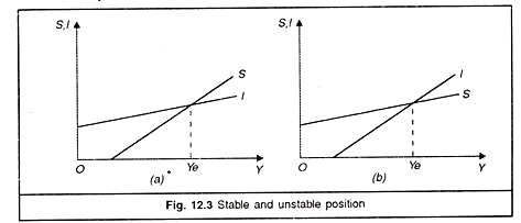
The first possibility is shown in Fig. 12.3(a) where the equilibrium is Y_e income level. When we assume linear S and I functions, there is a single equilibrium position and any disturbance that results in a shift in either function or both would tend to be followed by a movement to a new equilibrium position. This prevailing model shows more stability than appears to be in the real world.

In part (b) there is again a single equilibrium position but it is unstable one. Any disturbance producing a movement above Y means that 1 > S and that the income level may rise without limit. Any disturbance leading to a movement below Y>Y_e a movement below Y > Y_e means S > I and that the income level would collapse to zero. Part B gives us greater instability than the real world shows.

From this, Kaldor, therefore, concludes that S and I functions cannot both be linear, at least not over the full range of incomes during the business cycle. His opinion was that non-linear S and I functions appear to conform more closely to the behaviour of saving and investment in the course of a business cycle.

Kaldor’s Proposed Non-linear S and I Functions:

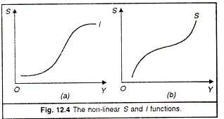
Refer to Figure 12.4. In part (a) the curve is almost flat for both relatively high and low income levels. This implies that the marginal propensity to invest, MPI is almost zero. The MPI is expected to be about zero at low income levels because there is already large excess capacity and rise in income at low rate will not induce any investment spending. Similarly, in case of high level of income, MPI will be small because of rising costs of construction and borrowing.

This will discourage entrepreneurs to invest more. In part (b) of the figure at relatively high and low income levels, the MPS, marginal propensity to save, is relatively large compared to its magnitude at normal income levels. During recession when incomes fall to low levels, people cut saving to maintain their previous standards of living and at high income levels, people not only save a large amount but also a larger proportion of their income. Therefore, the MPS is high both in a recession and a boom.

This shifts the distribution of income in favour of profits and away from wages because the MPS of profit seekers is higher than that of the wage earners. This is reflected in a steep rise of the S function at high income levels.

The Model:

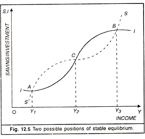
The adjoining figure 12.5 has been derived by combining the nonlinear I and S functions. This figure shows multiple equilibria of income with both A and B as stable positions. At income levels below Y₁, I> S, so the income level rises. At income levels between Y₁ and Y₂, S > I, so the income level falls. C is an unstable position and, therefore Y₂ is not a stable income level. If income happens to be between Y₂ and Y₃, it will rise to Y₃, and if income is between Y₁ and Y₂, it will fall to Y₃. It shows that the economy can reach stability either at some high level of income or at some low level of income Y₁.

This, however, does not give us a complete model of the business cycle, because a business cycle is made up of alternating expansions and contractions and this figure simply shows two possible positions of stable equilibrium. According to Kaldor, “The key to the explanation of the trade cycle is to be found in the fact that each of these two positions is stable only in the short period—that as activity continues at either one of these levels, forces gradually accumulate which sooner or later will render that particular position unstable.” If it can be shown that the stable equilibrium at A becomes unstable over time and forces a movement to B, we will have given the basic genesis of the business cycle.

 

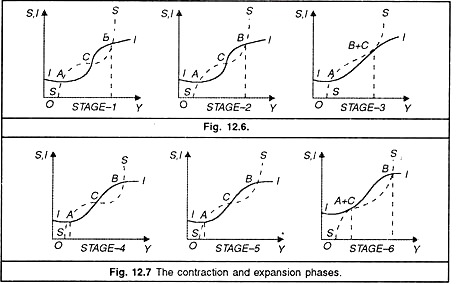
Kaldor argnes about the onset of contraction and expansion with a series of diagrams. In Figure 12.4 we start off our analysis with the assumption that the economy is in. equilibrium position at B, which corresponds to a relatively high income, at which investment is also high. We have assumed that the higher the rate of investment, the more rapid is the increase in the size of the capital stock. As the capital stock grows, it means falling MEC, which in turn leads to downward shift in the ME1 curve.

This is denoted here by a downward shift in the I curve (beyond point B). At the same time, the growth in the capital stock of the economy means a growth in the total wealth of the economy. This will tend to push up the saving curve beyond point B in stage 1 of this figure. This means that there is a rise in the average propensity to save in the economy induced by an increase in its wealth. As shown by stage 2 of the diagram, the downward movement of the I curve and the upward movement of S curve result in a gradual shift to the left of the position of B and a gradual shift in the position of C to the right until B and C are brought close to each other. The critical point is reached when these gradual shifts of the I and S curves make the two curves tangential to each other at point B. This will bring B and C together as is shown in stage 3 of the diagram. Now, at the position of B + C, S > I in both directions.

This implies that the equilibrium is unstable, that the income will move in a downward direction. The cyclical contraction, once started reduces the income level until a new stable equilibrium is reached at the relatively lower level that corresponds with A.

It may be noted that even position is of stable equilibrium income only in the short run. As time passes the S and I curves gradually shift. For the economy is at a relatively low income level, the I curve shifts upward and the S curve shifts downward, as is shown by stage 4 in the diagram. If the level of investment corresponding to A is less than the replacement requirements, some inward shift in the I curve would occur on account of replacement reasons alone. Besides as time passes, more investment opportunities develop pushing up the MEI curve.

This means an upward shift in the I curve. At the same time, any decline in the capital stock of the economy that occurs during the period of low income will tend to lower the average propensity to save. This will push the S curve downward. These shifts cause the position of A to move to the right and that of C to move to the left, thereby bringing A and C together as is shown in stage 4 and stage 5 in the diagrams.

In the process, the critical point is reached when these gradual shifts of the I and S curves make the two curves tangential that bring A and C together, as is shown in stage 6 of the diagram. The + C position is unstable as income goes in an upward direction, since I > S on both sides. The expansion, once started, raises the income level where a new state of equilibrium is reached at the position B. The S&I curves thereafter are likely to return gradually to the position shown in stage 1 of the diagram and another cycle begins.

The cyclical process described by Kaldor is thus self-generating. The very movement to relatively high income levels brings into play forces which with the passage of time have produced a downward movement to relatively low income levels, as the changing APS and the accumulation or decumulation of capital that occur over the cycle are inherent in the capitalist economic process. They are endogenous forces in the full sense of the term.

Besides the switching of the S & I functions, Kaldor’s model of trade cycle introduces the importance of the distribution of income. He contended that the income of the society is distributed between two classes of workers and employers as wages and profits each of which has its own propensity to save, while the relations of income distribution determine the level of saving, achievement of equilibrium requires a matching level of investment.

According to Kaldor, the introduction of the distribution mechanism (of income) into the model (with the provision that profit seekers’ savings are more than those of wage earners) makes the system more stable and more capable of automatically restoring equilibrium. Thus we find that Kaldor’s model differs materially from Harrod’s model. Kaldor believes that any change in I in relation to S— which in Harrod’s model will tend to produce cumulative processes of decline or growth in income will set off in Kaldor’s model the mechanism of income redistribution which adjusts S to the changed level of I.

Inflationary processes have an important part to play in this redistribution of income. Kaldor assumes that when I > S, the growth of demand under increased employment will result in faster growth of prices than of wages, thereby changing the distribution of income in favour of profit earners reducing the share of workers. Because savings from profits are assumed to be higher than the savings from wages (Sp > Sw) this will result in a growth of savings and the equality of S and I will be restored.

If, on the other hand, investment demand tends to decline, prices are likely to drop faster than wages, income distribution will tend to change in favour of the workers, savings will decline till the equality of S and I is restored. The stabilising effect which works through the mechanism of income distribution is called ‘Kaldor effect’.

According to Kaldor, the forces which bring about the lower turning point are not so strong at the higher level of income. “A boom left to itself is certain to come to an end, but the depression might get into a position of stationariness and remain there until external changes (the discovery of new inventions or of the opening of new markets) come to the rescue.”

Kaldor has observed also that cycles in his model are not of the same duration. Neither are expansions and contractions necessarily symmetrical. These attributes of the cycles depend upon the slopes of the I and S curves and the rate at which they shift in the course of the trade cycle.

Kaldor’s trade cycle model is unique in nature. He has neither used the acceleration principle nor the monetary factors in explaining the turning points of the trade cycle. He has used the existence of non-linear S and I functions along with the income distribution mechanism to demonstrate the generation of a business cycle.