In this article we will discuss about wage determination under non-pure competition.
The Marginal Productivity Theory of Distribution, as explained by J. B. Clark and others, is applicable in the case of factor-price (or labour-price i.e., wages) determination under pure competition. But, Mrs. Robinson and others have modified the theory to apply it in the case of factor-price determination under non-pure competition and monopoly.
As applied to wage determination under non-pure competition and monopoly, the theory can be explained as follows:
In the original theory it is stated that wages of labour become equal to the value of the marginal product of labour (VMPL). But, in the modified theory it is stated that an employer would employ labour up to that number at which wages (i.e., marginal wages) become equal to the marginal revenue product of labour (MRPL). Under pure competition, as price and marginal revenue are equal, the ‘value of marginal product of labour’ becomes equal to the ‘marginal revenue product of labour’ (VMPL=MRPL).
ADVERTISEMENTS:
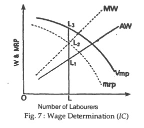
The modified theory also states that under non-pure competition the MRPL should be equal to marginal wages (not to average wages) for profit maximisation. Under pure competition, as the wage-rate remains constant for all labour, the average wages (AW) become equal to marginal wages (See WW’ line in Fig. 7). Owing to this reason, in equilibrium when the MRPL becomes equal to MW, it automatically becomes equal to AW.
But, as under non-pure competition and monopoly the rate of wages increases with the increase in the number of labour employed, MW becomes greater than AW, and so the MW curve will lie above the AW curve.
An employer under non-pure competition and monopoly, would employ the labour upto that number at which marginal wages become equal to the marginal revenue product of labour (MW=MRPL). But all the workers being homogeneous are to be paid at the same rate of wages; the determined wages would be less than both MRPL and VMPL. This can be seen from Fig. 7.
In Fig. 7 VMP curve is the value of marginal product curve of labour and MRP curve is the marginal revenue product curve of labour under non-pure competition or monopoly. As in such a situation MR<P the MRP curve lies below the VMP curve. In Fig.7, the AW curve and the MW curve are the average wage curve, and the marginal wage curves respectively. M W curve lies above A W curve, because here M W = MRPL But here the wage-rate (i.e., AW) is LL1.
ADVERTISEMENTS:
This rate of wages is less than MRPL which is LL2 and still less than VMPL by greater amount which is LL3 in the figure So, here wages are not equal to VMPL as ought to be in accordance with the marginal productivity theory. Here, the labour is getting less by L2L3 per unit of labour and this represents the exploitation per unit of labour by the employer.
This point may also be illustrated in another way, assuming monopoly in the product market.
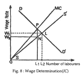
In Fig. 8 DD’ curve shows the MRPL of a monopoly firm. The curve SS’ is the average cost or average wage curve and MC curve is the marginal cost or the marginal wage curve. For profit maximisation the monopolist would employ labour up to that point where marginal cost (i.e., marginal wages) becomes equal to MRPL.
In the figure, it is seen that when OL2 labour is employed, the marginal cost (i.e., MW) becomes equal to the MRPL (i.e., at P—the point of intersection of MC curve and DD’ curve). So, the employer would employ OL2 number of labour are willing supply their services at wage-rate of OW2. In the case of perfect or pure competition, the employment will be OQ1 at the wage rate of O W2 or L2L. We see that in monopoly both wages and employment are less than those under perfect competition.
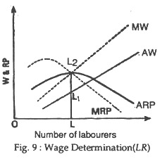
In the long run, as in the perfect competition and monopoly are equal to both marginal revenue product of labour and average revenue product (ARP) of labour as can be seen from Fig. 9.
The above figure shows that the employer in the long run under non- pure competition would employ OL number of labour because here MW (LL2) = MRPL (LL2) = ARPL (LL2). Here, wage rate or A W is LL1.


