Maximisation of Social Welfare | Economics

We shall now attempt to derive the conditions of social welfare maximisation in the simple two-factor, two-commodity, two-consumer model.

The Assumptions of Social Welfare :

Our analysis will be based on the following assumptions:

(i) There are two factors X₁ and X₂. Their quantities are given and constant, i.e., their supply is perfectly inelastic. These factors are homogeneous and perfectly divisible.

(ii) There are two commodities, Q₁ and Q₂ that are produced by two firms. Each firm produces only one commodity. The production functions give us smooth isoquants, convex to the origin, with constant returns to scale. Indivisibilities in the production processes are assumed away.

(iii) There are two consumers, I and II, whose preferences are represented by indifference curves that are continuous, convex to the origin and non-intersecting.

(iv) The goal of the consumers is utility maximisation and that of the firms is profit maximisation.

(v) The production functions are independent, i.e., the joint products and external economies and diseconomies in production are ruled out.

(vi) The utilities of consumers are independent. Bandwagon, Snob and Veblen effects are ruled out. There are no external economies or diseconomies in consumption.

(vii) The ownership of factors, i.e., the distribution of the given quantities of X₁ and X₂ between the two consumers, is exogenously determined.

(viii) A social welfare function, W = f (U_I, U_II) exists. On the basis of this function we shall be able to have a unique preference ordering of all possible economic states, based on the positions of the two consumers in their own preference maps. This welfare function incorporates an ethical valuation of the relative deservingness or worthiness of the two consumers.

The Values to be Obtained:

Our problem here is to determine the welfare-maximising values of the following variables:

(a) The welfare-maximising commodity-mix, i.e., the quantities of q₁ and q₂ of the goods Q₁ and Q₂ (production problem).

(b) The welfare-maximising distribution of the commodities produced, between the two consumers, i.e., the values of q₁₁, q₁₂, q₂₁, q₂₂ (distribution problem).

(c) The welfare-maximising allocation of the given resources in the production of Q₁ and Q₂, i.e., we have to determine the welfare-maximising values of x₁₁, x₁₂, x₂₁, x₂₂ (allocation problem).

That is, in the 2 x 2 x 2 model, we have ten unknowns, and we have to find the values of these unknowns which maximise the social welfare.

The tools that we would use in finding the situation where social welfare is maximised are:

(i) The social welfare function (SWF); and

(ii) The grand utility possibility frontier (GUPF).

  The latter shows the maximum utility attainable by individual II (or I), given the utility enjoyed by individual I (or II), for any given product-mix.

Utility Possibility Frontier (UPF) and the Grand Utility Possibility Frontier (GUPF):

Each product-mix, i.e., any particular combination of the goods Q₁ and Q₂, can be optimally distributed among the two consumers, I and II, in an infinite number of ways represented by the points on the Edge-worth contract curve for exchange or consumption (CCE or CCC) obtained for that combination.

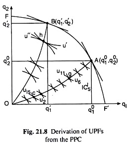
Let us take, for example, the combination of goods A(q⁰₁, q⁰₂) on the economy’s production possibility curve (PPC), FF’, in Fig. 21.8. Each point on the CCE, OA, represents a different distribution of Q₁ and Q₂ between the two consumers, and hence, a different combination of utilities of the two consumers.

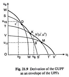
For example, the point c denotes the combination of utility level, u₂ of consumer I and u₁₅ of consumer II. We can plot this utility combination as a point in the utility space given in Fig. 21.9. Let us suppose, this point is c’.

We may repeat the process again to obtain another combination of utilities of the two consumers. For example, corresponding to the point g on the CCE in Fig. 21.8, we may obtain a point like g’ in Fig. 21.9 where U_I is greater and U_II is smaller.

Points c’ and g’ give us, respectively, the maximum utility that individual II may obtain corresponding to the given level of utility of individual I, or the other way round. We may also note here that we have mapped points c and g on the CCE, OA, in Fig. 21.8, into the points c’ and g’ in Fig. 21.9.

In the same way, we may map as many points of the CCE as we like into the utility space of Fig. 21.9. If we join these points including the points c’ and g’ by a curve (here SS’), then we obtain what is called a utility possibility frontier (UPF). In other words, what we have seen is that any particular CCE corresponding to a particular product-mix on the PPC may give rise to a particular UPF.

Therefore, an infinitely large number of points on the PPC would give us an infinitely large number of UPFs. It may be noted here that the UPFs will be negatively sloped, for along each UPF, as U_I increases, U_II decreases as obtained from the corresponding movement along the Edge-worth CCE.

Now, if we consider any particular UPF, we find what the maximum U_II would be corresponding to a given U] along that UPF. But this maximum U_II corresponding to a given U_I may be different for different UPFs. For example, in Fig. 21.9, we have shown some of the UPFs corresponding to different points on the PPC. These UPFs are WW’, SS’, TT’ and VV’. Now for any given level of u_I = u₆, we have u_II = u₁₁ at the point g’ on the UPF, SS’. But at the same level of U_I, U_II is larger at the point h’ on the UPF, TT’.

Therefore, at any given level of U_I, the maximum possible u_II would be given by the envelope of all the possible UPFs. This envelope is known as the grand utility possibility frontier (GUPF). GUPF gives us what would be the maximum possible u_II at any given u_I if we consider not any one UPF but all the UPFs that may be obtained for the different combinations of the goods on the PPC.

Similarly, it would give us what would be the maximum possible u_I at any given u_II, considering all the UPFs that may be generated by the points on the PPC. The GUPF that may be derived from the PPC given in Fig. 21.8 would be like the kinked path WDKMV’ in Fig. 21.9—it would be made up of four scallops one from each of the four UPFs.

An Alternative Way of Obtaining the GUPF:

We may derive the GUPF in an alternative way by using the third marginal condition of Pareto optimality. This condition states that the MRS of Q₁ for Q₂ for each consumer should be equal to the MRPT of Q₂ into Q₁. Let us suppose that at the point A(q⁰₁, q⁰₂) on the economy’s PPC in Fig. 21.8, the Edge-worth CCE is OA, and at the point c on OA, the common slope of the tangent IQs is equal to the slope of the PPC at the point A.

This gives us that at the product-mix A(q⁰₁, q⁰₂), the MRPT of Q₂ into Q₁ has been equal to the MRS of Q₁ for Q₂ of each consumer, i.e., the third condition of the Pareto-optimality has been satisfied at the product-mix A(q’₁, q’₂) or, at the implicitly obtained combination c (u₂, u₁₅) of utilities of the two individuals on the Edge-worth CCE.

At c (u₂, u₁₅) goods have been distributed between the two consumers in such a way that by no further redistribution, utility of one of them can be increased without reducing the utility of the other, i.e., utility of one of them is maximum at the given level of utility of the other. In other words, the point c'(u₂, u₁₅) in the utility space of Fig. 21.9 lies on the GUPF.

Similarly, at the point B (q’₁, q’₂) on the PPC, the Edge-worth CCE is OB, and at the point h on OB, the common slope of the tangent IQs has been equal to the slope of the PPC at the point B (q₁, q₂).

In other words, at the product-mix B (q₁, q₂), the MRPT of Q₁ into Q₂ has been equal to MRS of Q₁ for Q₂ of each consumer, i.e., the third condition of Pareto-optimality has been satisfied for the product-mix B(q₁,q₂) at the implicitly obtained utility combination h (u’, u”) of the two individuals.

In other words, the point h’ (u’, u”) in the utility space of Fig. 21.9 lies on the GUPF. Just like c’ and h’, we may have many other points on the GUPF of the economy, and by joining these points we would be able to derive the required GUPF.

Let us remember here that each point or the utility combination of the two individuals on the GUPF satisfies all the three Pareto-optimality conditions. To understand this, let us take any point c'(u₂,u₁₅) on the GUPF. The utility combination (u₂, u₁₅) at c’ is obtained at the point c on the Edge-worth CCE, OA, in Fig. 21.8.

Therefore, the utility combination at the point c’ on GUPF satisfies the Pareto-optimality condition for exchange. Second, the utility combination at c’ emerges out of a distribution of the product-mix A(q⁰₁, q⁰₂) on the PPC between the two consumers.

Since the points on the PPC correspond on a one-to-one basis to the points on the Edge-worth CCP (contract curve for production), the point A on the PPC and, therefore, the point c'(u₂, u₁₅) on the GUPF satisfies the Pareto-optimality condition for production. Third, the common slope of the tangent IQs at the point c on the CCE, OA, in Fig. 21.8, is equal to the slope of the PPC at the point A.

This implies that the point c or the utility combination (u₂, u₁₅) implicitly obtained at the point c, and so, the point c'(u₂,u₁₅) on the GUPF, satisfies the third Pareto-optimality condition for product-mix which states that MRPT of Q₂ into Q₁ should be equal to MRS_Q1,Q2 for each consumer.

Determination of the Welfare-Maximising State:

The tools that would be used in finding the situation where social welfare is maximised are:

(i) The social welfare function (SWF) that gives us the social indifference map of the economy; and

(ii) The grand utility possibility frontier (GUPF) given by the PPC of the economy.

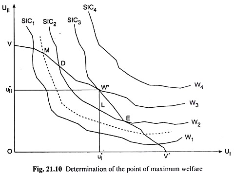
In Fig. 21.10, we have combined the social indifference contours (SICs) and the GUPF. As the name suggests and as we have seen, the GUPF gives us the utility possibilities- the maximum u_II subject to any given u_I or the maximum u_I subject to any given u_II—that the society can reach. The social welfare has to be maximised subject to these utility possibilities.

That is, white remaining on the GUPF, the society should attempt to reach the highest possible social indifference contour. This the society would achieve, i.e., social welfare would be maximised at the point of tangency between the GUPF and one of the SICs.

In Fig. 21.10, this point of tangency—or the social welfare maximising point—is given by W*. This is called the point of bliss. At this point (W*) in Fig. 21.10 the social welfare level that can be attained is W₃ and the highest possible SIC has been SIC₃. At W* the utilities obtained by the two individuals are u*_I and u*_II, respectively.